• Photonics Research
  • Vol. 9, Issue 9, 1842 (2021)
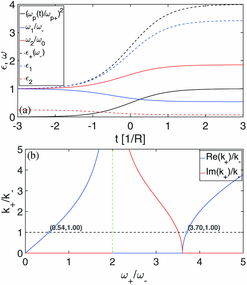
Diego M. Solís1, Raphael Kastner1、2, and Nader Engheta1、*
Author Affiliations
  • 1Department of Electrical and Systems Engineering, University of Pennsylvania, Philadelphia, Pennsylvania 19104, USA
  • 2Tel Aviv University, Tel Aviv 69978, Israel
  • show less
    DOI: 10.1364/PRJ.427368 Cite this Article Set citation alerts
    Diego M. Solís, Raphael Kastner, Nader Engheta. Time-varying materials in the presence of dispersion: plane-wave propagation in a Lorentzian medium with temporal discontinuity[J]. Photonics Research, 2021, 9(9): 1842 Copy Citation Text show less
    (a) Temporal evolution of ωl and ϵl (l=1,2) as ωp(t) transitions from ωp−=0 (vacuum) to ωp+ such that ϵ+(ω−)=4 with ω0=2ω−, resulting in ωp+=3ω−. (b) Dispersion diagram k+ versus ω+, showing the two solutions for ω+ that achieve momentum conservation. The dashed green line represents ω0.
    Fig. 1. (a) Temporal evolution of ωl and ϵl (l=1,2) as ωp(t) transitions from ωp=0 (vacuum) to ωp+ such that ϵ+(ω)=4 with ω0=2ω, resulting in ωp+=3ω. (b) Dispersion diagram k+ versus ω+, showing the two solutions for ω+ that achieve momentum conservation. The dashed green line represents ω0.
    (a) Electromagnetic waves versus time at z=λ/16 for a transition from ϵ−(ω−)=1 (vacuum) to ϵ+(ω−)=4, with ω0=2ω− (the solid lines are analytical results, while the circular markers represent numerical FDTD simulations). (b1) New frequencies ωi [and ϵ+(ωi)] for t>0 and (b2) wave amplitude coefficients versus ω0/ω−, considering ωp+=3ω− [ϵ+(ω−)→1 as ω0/ω−→∞]. Panels (c1), (c2) are the same, but with ϵ+(ω−)=4 [ωp+→χ+(ω−)ω0 as ω0/ω−→∞].
    Fig. 2. (a) Electromagnetic waves versus time at z=λ/16 for a transition from ϵ(ω)=1 (vacuum) to ϵ+(ω)=4, with ω0=2ω (the solid lines are analytical results, while the circular markers represent numerical FDTD simulations). (b1) New frequencies ωi [and ϵ+(ωi)] for t>0 and (b2) wave amplitude coefficients versus ω0/ω, considering ωp+=3ω [ϵ+(ω)1 as ω0/ω]. Panels (c1), (c2) are the same, but with ϵ+(ω)=4 [ωp+χ+(ω)ω0 as ω0/ω].
    Transmission-line equivalence of our unbounded time-varying dispersive medium. At t=0, the switch is closed, effectively connecting our series tank circuit LpCp.
    Fig. 3. Transmission-line equivalence of our unbounded time-varying dispersive medium. At t=0, the switch is closed, effectively connecting our series tank circuit LpCp.
    (a) Dispersion diagram in the complex k- and ω-planes when ϵ+(ω−)=4−0.1i, which results in ωp+≈3ω− and γ=0.1ω− when ω0=2ω−. Conservation of momentum is achieved when the surfaces [ω+,Re[k+(ω+)]/k−] and [ω+,Im[k+(ω+)]/k−] simultaneously intersect the Re(k+)/k−=1 and Im(k+)/k−=0 planes (gray color), respectively. These intersection curves are marked in black and give rise to four complex frequencies that, in this example, form two complex-conjugate pairs in the s plane [the plotted region Re(ω+)>0 only includes one complex frequency per pair]. (b) Evolution of the four complex frequencies versus γ, with the other parameters fixed [ω0 and ωp+ from panel (a)]: at γ=7.01ω− we reach a critical point, and the pair of complex frequencies linked to ω0 (ω2f and ω2b) splits into two purely imaginary frequencies for which ϵ becomes purely real and negative; the latter is seen in panel (c). Note that, in this overdamped region (γ>7.01ω−), the notation ω2f and ω2b is not strictly rigorous: this pair simply becomes ω2 and ω3, and the associated waves represent non-propagating damping.
    Fig. 4. (a) Dispersion diagram in the complex k- and ω-planes when ϵ+(ω)=40.1i, which results in ωp+3ω and γ=0.1ω when ω0=2ω. Conservation of momentum is achieved when the surfaces [ω+,Re[k+(ω+)]/k] and [ω+,Im[k+(ω+)]/k] simultaneously intersect the Re(k+)/k=1 and Im(k+)/k=0 planes (gray color), respectively. These intersection curves are marked in black and give rise to four complex frequencies that, in this example, form two complex-conjugate pairs in the s plane [the plotted region Re(ω+)>0 only includes one complex frequency per pair]. (b) Evolution of the four complex frequencies versus γ, with the other parameters fixed [ω0 and ωp+ from panel (a)]: at γ=7.01ω we reach a critical point, and the pair of complex frequencies linked to ω0 (ω2f and ω2b) splits into two purely imaginary frequencies for which ϵ becomes purely real and negative; the latter is seen in panel (c). Note that, in this overdamped region (γ>7.01ω), the notation ω2f and ω2b is not strictly rigorous: this pair simply becomes ω2 and ω3, and the associated waves represent non-propagating damping.
    (a) Electromagnetic waves versus time at z=λ/16 when ω0 and ωp+ are taken from Fig. 4 and γ=0.5ω− (numerical FDTD simulations are marked with circles): we have ω2f and ω2b, corresponding to an underdamped scenario. (b) Separate components of E(z=0,t>0). (c) Two snapshots of the separate components of E+ [the solid and dashed lines represent E(z,t=0+) and E(z,t=T/32), respectively], showing forward and backward propagation for both ω1 and ω2.
    Fig. 5. (a) Electromagnetic waves versus time at z=λ/16 when ω0 and ωp+ are taken from Fig. 4 and γ=0.5ω (numerical FDTD simulations are marked with circles): we have ω2f and ω2b, corresponding to an underdamped scenario. (b) Separate components of E(z=0,t>0). (c) Two snapshots of the separate components of E+ [the solid and dashed lines represent E(z,t=0+) and E(z,t=T/32), respectively], showing forward and backward propagation for both ω1 and ω2.
    Same as Fig. 5 but with γ=7.3ω−, yielding an overdamped regime with purely imaginary ω2 and ω3 describing oscillations that do not propagate. This is seen in panel (c): red (E2) and green (E3) curves.
    Fig. 6. Same as Fig. 5 but with γ=7.3ω, yielding an overdamped regime with purely imaginary ω2 and ω3 describing oscillations that do not propagate. This is seen in panel (c): red (E2) and green (E3) curves.
    Real and imaginary parts of the complex amplitude coefficients versus γ/ω−. As ω2f→ω2b near the point of critical damping γ=7.01ω−, f2 and b2 tend to diverge but with opposite signs [panel (b)], keeping f2+b2 (or else x2+x3) bounded.
    Fig. 7. Real and imaginary parts of the complex amplitude coefficients versus γ/ω. As ω2fω2b near the point of critical damping γ=7.01ω, f2 and b2 tend to diverge but with opposite signs [panel (b)], keeping f2+b2 (or else x2+x3) bounded.
    (a1) Normalized real and imaginary parts of the complex frequencies ω2f (ω2) and ω2b (ω3) versus ω0χi/ω−, for χi=10−3 (lines) and χi=10−4 (markers). (a2) Normalized dielectric functions ϵ2f (ϵ2) and ϵ2b (ϵ3). (b) Complex amplitude coefficients f2 (x2) and b2 (x3). (c) E2f (E3) and E2b (E3) versus normalized time, for z=0 and several ω0/ω− ratios; note how the black and red plots, corresponding to the underdamped region where f2=b2, are superimposed.
    Fig. 8. (a1) Normalized real and imaginary parts of the complex frequencies ω2f (ω2) and ω2b (ω3) versus ω0χi/ω, for χi=103 (lines) and χi=104 (markers). (a2) Normalized dielectric functions ϵ2f (ϵ2) and ϵ2b (ϵ3). (b) Complex amplitude coefficients f2 (x2) and b2 (x3). (c) E2f (E3) and E2b (E3) versus normalized time, for z=0 and several ω0/ω ratios; note how the black and red plots, corresponding to the underdamped region where f2=b2, are superimposed.
    (a) Electromagnetic waves versus time at z=λ/16 for the transition from vacuum to ϵ+(ω−)=4−iχi, considering ω0=104ω− and several values of χi specified in panel (b); all the curves are virtually the same and overlap with the chosen t-axis scale, converging to the solution of the nondispersive lossless case. (b) Zoomed-in view of the transition of panel (a), both for underdamped (solid lines) and overdamped (dashed lines) scenarios.
    Fig. 9. (a) Electromagnetic waves versus time at z=λ/16 for the transition from vacuum to ϵ+(ω)=4iχi, considering ω0=104ω and several values of χi specified in panel (b); all the curves are virtually the same and overlap with the chosen t-axis scale, converging to the solution of the nondispersive lossless case. (b) Zoomed-in view of the transition of panel (a), both for underdamped (solid lines) and overdamped (dashed lines) scenarios.
    Diego M. Solís, Raphael Kastner, Nader Engheta. Time-varying materials in the presence of dispersion: plane-wave propagation in a Lorentzian medium with temporal discontinuity[J]. Photonics Research, 2021, 9(9): 1842
    Download Citation