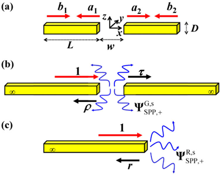
Fig. 1. (a) Sketch of the nanogap antenna. The antenna is composed of two gold nanowire arms of length L (with a square cross section of side length D=40  nm) separated by a nanogap (gap width w=30  nm). a1, a2, b1, and b2 are the complex amplitude coefficients of SPPs at the complex eigenfrequency of QNMs. (b) and (c) definitions of SPP scattering coefficients ρ, τ, and r and scattered fields ΨSPP,+G,s and ΨSPP,+R,s used in the model.

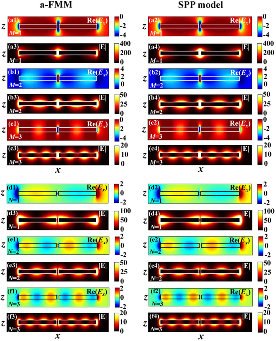
Fig. 2. Field distributions of QNMs for antenna arm length L=0.6  μm. The left and right columns show the results obtained with the full-wave a-FMM and with the SPP model, respectively. (a)–(c) show the bonding QNMs for M=1, 2, 3, respectively, where the electric-field amplitude is defined as |E|=|Ex|2+|Ey|2+|Ez|2. (d)–(f) show the antibonding QNMs for N=1, 2, 3, respectively.

Fig. 3. (a) Definitions of the amplitude coefficients (c1, c2, d1, and d2) of SPPs excited by an x-polarized electric point source located at the center of the nanogap. (b) Definitions of the SPP excitation coefficient β and scattered field used in the model. (c) Enhancement factor F of radiation plotted as a function of illumination frequency ω/(2πc). Results are obtained with the full-wave a-FMM (blue circles) and the SPP model (red solid curve) for antenna length L=0.6  μm.

Fig. 4. (a) Definitions of the amplitude coefficients (e1, e2, f1, and f2) of SPPs excited by an x-polarized electric point source located near the antenna termination (with a distance of 15 nm). (b) Definitions of the SPP excitation coefficient α and scattered field ΨSourceT used in the model. (c) Enhancement factor F of radiation plotted as a function of illumination frequency ω/(2πc). Results are obtained with the full-wave a-FMM (blue circles) and the SPP model (red-solid curve), with antenna length L=0.6  μm.

Fig. 5. SPP field and the residual field on the surface of the antenna arms for different orders of QNMs. (a1) and (a2) correspond to M=1 and M=2 orders of bonding QNMs, respectively. (b1) and (b2) correspond to N=1 and N=2 orders of antibonding QNMs, respectively. The results are obtained for antenna length L=0.6  μm.

Fig. 6. SPP field and the residual field on the surface of the antenna arms at different resonance peaks of the enhancement factor F of radiation plotted in Figs. 3(c) and 4(c). (a1) and (a2) show the results at resonances corresponding to the M=1 and M=2 orders of QNMs for the case that the source is located at the center of the nanogap [see Fig. 3(c)]. (b1), (b2), (c1), and (c2) show the results at the resonances corresponding to M=1, 2 and N=1, 2 orders of QNMs for the case that the source is located near the antenna termination [see Fig. 4(c)]. The results are obtained for antenna length L=0.6  μm.

Fig. 7. Field distributions of QNMs for antenna length L=0.2  μm. The left and right columns show the results obtained with the full-wave a-FMM and with the SPP model, respectively. (a) and (b) show the real part of Ex component and the amplitude of the electric field (|E|=|Ex|2+|Ey|2+|Ez|2) for the M=1 order QNM. (c) and (d) show the results for the N=1 order QNM.

Fig. 8. Enhancement factor F of radiation plotted as a function of illumination frequency ω/(2πc) for antenna length L=0.2  μm. The results are obtained with the full-wave a-FMM (blue circles) and the SPP model (red solid curves). (a) is for the case that the point emitter is located at the gap center [as sketched in Fig. 3(a)]. (b) is for the case that the point emitter is located near the antenna termination [as sketched in Fig. 4(a)].

Fig. 9. Calculation of the SPP excitation coefficients β and α with the Lorentzian reciprocity theorem. (a) and (c) Definitions of the SPP excitation coefficients for the point emitter located in the nanogap and near the antenna termination, respectively. (b) and (d) Reciprocal scattering processes of (a) and (c) by sending an incident SPP toward the nanogap and toward the antenna termination, respectively. ESPP,+G,tot(r0) and ESPP,+R,tot(r0) in (b) and (d) denote the electric field at the source position r0 excited by the incident SPP.

Fig. 10. (a) Total field ΨSPP,+G,tot excited by a right-going SPP incident from the left arm of an infinitely long nanowire with a nanogap. (b) Incident right-going SPP field ΨSPP,+G,inc in the absence of the scatterer of the nanogap. (c) Total field ΨSPP,+R,tot excited by a right-going SPP at a right-terminated semi-infinitely long nanowire. (d) Incident right-going SPP field ΨSPP,+R,inc at an infinitely long nanowire. (e)–(h) The same as (a)–(d) but for a left-going incident SPP.

Table 1. Complex Eigenfrequencies ωc (λc=2πc/ωc) of QNMs