Improving the resolution in quantum and classical temporal imaging

Junheng Shi; Giuseppe Patera; Youzhen Gui; Mikhail I. Kolobov; Dmitri B. Horoshko; Shensheng Han

doi:10.3788/COL201816.092701

Abstract

The point-spread function of an optical system determines its optical resolution for both spatial and temporal imaging. For spatial imaging, it is given by a Fourier transform of the pupil function of the system. For temporal imaging based on nonlinear optical processes, such as sum-frequency generation or four-wave mixing, the point-spread function is related to the waveform of the pump wave by a nonlinear transformation. We compare the point-spread functions of three temporal imaging schemes: sum-frequency generation, co-propagating four-wave mixing, and counter-propagating four-wave mixing, and demonstrate that the last scheme provides the best temporal resolution. Our results are valid for both quantum and classical temporal imaging.

Temporal imaging is a technique for manipulating temporal waveforms of optical signals similar to the manipulation of spatial wavefronts in conventional spatial imaging. It is based on the space–time analogy, i.e., equivalence of the phenomena of wave propagation in dispersive media and wave diffraction in free space^[1]. In the last decades, temporal imaging has been growing very rapidly with numerous applications from stretching of ultrafast waveforms and compression of slow waveforms, to temporal microscopes, time reversal, and spectral phase conjugation^[2].

The key element of a temporal imaging system is a time lens, introducing a quadratic in-time phase modulation into a temporal waveform similarly to its spatial counterpart. Optical time lenses have been realized using electro-optical phase modulation^[3–7], sum-frequency generation (SFG)^[8,9], and four-wave mixing (FWM)^[10–13].

Almost all applications of temporal imaging have been applied to classical optical fields and did neglect their quantum nature. However, temporal imaging has many potential applications in quantum optics and quantum information. For instance, it should allow for noiseless compression or stretching of nonclassical waveforms without destroying their quantum features. Such applications of quantum temporal imaging still are waiting for their experimental demonstrations, and only a few papers have addressed the subject so far. Some aspects of temporal imaging for nonclassical states of light with a few photons were considered in Refs. [7,14–17]. Quantum temporal imaging of broadband squeezed light was discussed in Refs. [18–20]. In particular, it was pointed out that special care must be taken for temporal imaging of squeezed light using SFG and FWM processes.

Sign up for Chinese Optics Letters TOC. Get the latest issue of Chinese Optics Letters delivered right to you！Sign up now

Optical resolution is one of the most important parameters characterizing an imaging system in both spatial and temporal imaging. It can be evaluated from the knowledge of its point-spread function, which describes the response of the system to a point-like object in space or time. It is well-known in spatial imaging that the resolution of an optical system is limited by diffraction and that the point-spread function of the system is given by a Fourier transform of its pupil function. In temporal imaging based on nonlinear optical phenomena, such as SFG or FWM, the situation is more complicated. Indeed, due to the nonlinear nature of the process, the point-spread function of a temporal imaging system in general is related to the temporal waveform of the pump wave by a nonlinear transformation. When the efficiency of nonlinear interaction is very small and one can use the linear approximation, the point-spread function is given by the Fourier transform of the pump profile^[21,22]. However, in this approximation the efficiency of the time lens is very small. This does not create particular problems for classical temporal imaging when the statistical properties of the transmitted light are not relevant. But, in quantum temporal imaging, the low efficiency of a lens is detrimental for the nonclassical features, such as squeezing, entanglement, or nonclassical photon statistics^[18–20]. Therefore, in quantum temporal imaging, one has to use the time lens with the efficiency close to unity , consequently, when the point-spread function is a nonlinear function of the pump profile.

In this Letter, we investigate three simple temporal imaging schemes based on nonlinear time lenses: SFG, co-propagating (CBS), and counter-propagating (CPBS) FWM of the Bragg-scattering type. We evaluate the pupil function in terms of the pump profile for these schemes and use the width of the corresponding point-spread functions as the resolution limit. We demonstrate that the counter-propagating FWM scheme provides the best choice in terms of the resolution. Even if we limit our consideration to the coherent input states of light, i.e., classical temporal imaging, our results remain valid for quantum temporal imaging because the relevant point-spread function is the same for both cases.

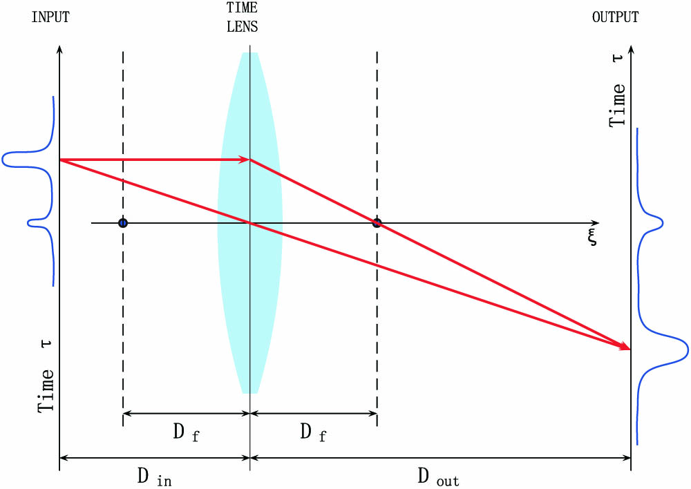
We consider a simple temporal imaging system shown in Fig. 1. It consists of a first dispersive medium followed by a time lens and the second dispersive medium. In the following, we will refer to the first (second) medium as the input (output) dispersive medium. The time lens is implemented by a nonlinear process that can be either SFG or FWM. In this section, we consider the SFG geometry, while the FWM case will be addressed in the next section. In the SFG process, a strong pump wave of frequency $ω_{p}$ is converted into a signal wave of the frequency $ω_{s}$ and the idler waves of the frequency $ω_{i}$ , such that $ω_{s} + ω_{p} = ω_{i}$ .

Figure 1.Temporal imaging system with a single time lens.

We use the plane-wave approximation and describe each field by its positive-frequency amplitude $E_{μ}^{(+)} (t, z)$ at the time $t$ and the longitudinal position $z$ , where the index $μ = {s, i, p}$ identifies the signal, the idler, or the pump waves, respectively. We consider the signal and the idler waves as quantum-mechanical operators and the pump wave as a classical $c$ function. All waves are assumed to be narrowband with the carrier frequencies $ω_{μ}$ . Each wave passing through a medium experiences dispersion characterized by the dependence of its wave vector $k_{μ} (ω)$ on frequency $ω$ , which we decompose around the carrier frequency at $Ω = ω - ω_{μ}$ and limit the Taylor series to the first three terms: $k_{μ} (ω) \approx k_{μ} (ω_{μ}) + β_{μ}^{(1)} Ω + β_{μ}^{(2)} Ω^{2} / 2,$ (1)where $β_{μ}^{(1)} = {(d k_{μ} / d Ω)}_{ω_{μ}}$ is the inverse group velocity, and $β_{μ}^{(2)} = {(d^{2} k_{μ} / d Ω^{2})}_{ω_{μ}}$ is the group velocity dispersion of the medium at the carrier frequency $ω_{μ}$ .

We introduce a frame of reference traveling with the wave at the group velocity, possibly different in each medium. Thus, for each point $z$ , we introduce the delayed time $τ = t - τ_{μ} (z)$ , where $τ_{μ} (z)$ is the total delay for the wave $E_{μ}^{(+)} (t, z)$ from the object plane at $z = z_{in}$ to the point $z$ between $z_{in}$ and the image plane $z = z_{out}$ . A delay in a medium of the length $l$ for the inverse group velocity $β_{μ}^{(1)}$ is $β_{μ}^{(1)} l$ , and the total delay $τ_{μ} (z)$ can be found by summing the delays of all media between $z_{in}$ and $z$ .

In this reference frame, we can write ${\hat{E}}_{μ}^{(+)} (t, z) = E_{μ} e^{i (k_{μ} z - ω_{μ} t)} {\hat{A}}_{μ} (τ, z),$ (2)where $E_{μ}$ is the single-photon field amplitude, $k_{μ} (ω_{μ}) = k_{μ}$ , and field envelope ${\hat{A}}_{μ} (τ, z)$ is given by ${\hat{A}}_{μ} (τ, z) = \frac{1}{2 π} \int_{- \infty}^{\infty} {\hat{ϵ}}_{μ} (Ω, z) e^{i β_{μ}^{(2)} Ω^{2} (z - z_{0}) / 2 - i Ω τ} d Ω,$ (3)with $\hat{ϵ} (Ω, z)$ being the slowly varying quantum amplitude^[23,24] for the given medium with the entrance point at $z_{0}$ .

Assuming the perfect phase matching and the undepleted pump, the SFG time lens can be described by the following unitary transformation from the point $z_{1}$ (time lens input) to the point $z_{2}$ (time lens output)^[18]: ${\hat{A}}_{s} (τ, z_{2}) = c (τ) {\hat{A}}_{s} (τ, z_{1}) - s (τ) e^{- i ϕ (τ)} {\hat{A}}_{i} (τ, z_{1}), {\hat{A}}_{i} (τ, z_{2}) = s (τ) e^{i ϕ (τ)} {\hat{A}}_{s} (τ, z_{1}) + c (τ) {\hat{A}}_{i} (τ, z_{1}),$ (4)with $c (τ) = \cos [g A_{p} (τ) L], s (τ) = \sin [g A_{p} (τ) L] .$ (5)

Here, $L = z_{2} - z_{1}$ is the length of the nonlinear medium, while $A_{p} (τ)$ and $ϕ (τ)$ are the modulus and phase of the pump pulse. For the implementation of a time lens, a short Gaussian pulse of duration $τ_{p}$ is propagated through a dispersive medium of length $L_{p}$ and group velocity dispersion $β_{p}^{(2)}$ at the carrier frequency $ω_{p}$ . At the output of the medium, the pump pulse is stretched to the duration $T ≫ τ_{p}$ and acquires a phase that is quadratic in time, $ϕ (τ) = τ^{2} / 2 D_{f}$ with $D_{f} = - β_{p}^{(2)} L_{p}$ known as the focal group delay dispersion (GDD)^[21,22]. In the present work, we consider only the case of negatively chirped pump $β_{p}^{(2)} < 0$ for definiteness. As a consequence, $D_{f} > 0$ . We also assume that the signal and the idler beams pass through the media with positive dispersion so that both $D_{in}$ and $D_{out}$ are positive.

Equation (4) describes a unitary transformation of the photon annihilation operators of the signal and the idler waves from the input of the SFG crystal to its output, preserving the canonical commutation relations. As follows from their definitions, the coefficients $c (τ)$ and $s (τ)$ satisfy the condition ${| c (τ) |}^{2} + {| s (τ) |}^{2} = 1.$ (6)

Therefore, they can be interpreted as the reflection and the transmission coefficients of an equivalent beam splitter. For time lens applications, the signal port is injected with an input state, while the input idler port is empty. As a consequence, the vacuum fluctuations enter into the process through this port and mix with the input state. Since these vacuum fluctuations are detrimental for the nonclassical input states, they need to be avoided. They can be eliminated by setting experimental conditions such that the conversion efficiency is $η = {| s (τ) |}^{2} = 1$ . This condition can be obtained by requiring $g A_{p} (τ) L = π / 2$ . However, since the pump pulses have a finite duration, the previous conditions cannot be satisfied for all $τ$ . The consequence is that the time lens presents a finite temporal aperture that lets in vacuum fluctuations.

Combining Eq. (4) with the free propagation in the dispersive media before and after the lens, we obtain the transformation of the field from the object plane to the image plane, ${\hat{A}}_{out} (τ) = \frac{i}{\sqrt{| M |}} \exp (- \frac{i τ^{2}}{2 | M | D_{f}}) \times [\int_{- \infty}^{\infty} \tilde{p} (τ, τ^{'}) {\hat{A}}_{in} (\frac{τ^{'}}{M}) d τ^{'} + \int_{- \infty}^{\infty} \tilde{q} (τ, τ^{'}) {\hat{B}}_{in} (\frac{τ^{'}}{M}) d τ^{'}],$ (7)where we have denoted ${\hat{A}}_{out} (τ) = {\hat{A}}_{i} (τ, z_{out})$ , ${\hat{A}}_{in} (τ) = {\hat{A}}_{s} (τ, z_{in})$ , and ${\hat{B}}_{in} (τ) = {\hat{A}}_{i} (τ, z_{in})$ . The last operator describes the vacuum field of the idler in the object plane and is absent in the classical temporal imaging theory. The impulse response functions $\tilde{p} (τ, τ^{'})$ and $\tilde{q} (τ, τ^{'})$ in Eq. (7) have the following form: $\tilde{p} (τ, τ^{'}) = p (τ - τ^{'}) e^{i θ (τ, τ^{'})},$ (8) $\tilde{q} (τ, τ^{'}) = q (τ - τ^{'}) e^{i θ (τ, τ^{'})},$ (9)where the function $p (τ)$ is the point-spread function of the classical imaging transformation^[1], $p (τ) = \frac{1}{2 π} \int_{- \infty}^{\infty} d Ω e^{i τ Ω} s (D_{out} Ω),$ (10)and the function $q (τ)$ is the second point-spread function necessary for the quantum description of our temporal imaging scheme. It describes the temporal imaging of the quantum fluctuations of the field ${\hat{B}}_{in} (τ)$ and is absent in the classical theory of temporal imaging because such fluctuations do not exist in the classical theory. This point-spread function is given by the following Fourier transform of the coefficient $c (τ)$ from Eq. (5), properly scaled and phase-adjusted as follows: $q (τ) = \frac{1}{2 π} \int_{- \infty}^{\infty} d Ω e^{i τ Ω} c^{'} (D_{out} Ω),$ (11)with $c^{'} (τ) = c (τ) \exp (- i τ^{2} / 2 D_{f})$ , and $θ (τ, τ^{'}) = \frac{τ^{2} - τ^{' 2}}{2 | M | D_{out}} .$ (12)

In derivation of Eqs. (8) and (9), we have used the time lens of Eq. (1), $\frac{1}{D_{in}} + \frac{1}{D_{out}} = \frac{1}{D_{f}},$ (13)and the definition of the magnification $M = - D_{out} / D_{in}$ .

The impulse response functions $\tilde{p} (τ, τ^{'})$ and $\tilde{q} (τ, τ^{'})$ satisfy the relation $\int_{- \infty}^{\infty} \tilde{p} (τ, s) {\tilde{p}}^{*} (τ^{'}, s) d s + \int_{- \infty}^{\infty} \tilde{q} (τ, s) {\tilde{q}}^{*} (τ^{'}, s) d s = δ (τ - τ^{'}),$ (14)required by the unitarity of Eq. (7).

While the transfer function $p (τ, τ^{'})$ is well-known in the classical temporal imaging theory^[1,21], the second term in Eq. (7) with the transfer function $q (τ, τ^{'})$ was introduced for the first time, to the best of our knowledge, in Ref. [25]. Using the time-invariant approximation as in Ref. [25], Eq. (7) can be rewritten in the following simple form: ${\hat{A}}_{out} (τ) = \frac{i}{\sqrt{| M |}} \exp (- \frac{i τ^{2}}{2 | M | D_{f}}) \times [\int_{- \infty}^{\infty} p (τ - τ^{'}) {\hat{A}}_{in} (\frac{τ^{'}}{M}) d τ^{'} + \int_{- \infty}^{\infty} q (τ - τ^{'}) {\hat{B}}_{in} (\frac{τ^{'}}{M}) d τ^{'}] .$ (15)

The overall transformation in Eq. (15) consists of three elementary transformations for each input field: (i) scaling of time with the factor $M$ , (ii) temporal convolution with a time-invariant transfer function, and (iii) multiplication by a quadratic in-time phase factor. In the next section, we show that such evolution corresponds to a simple transformation of the spectrum observed in a homodyne measurement with a properly chosen local oscillator.

In the limiting case of infinitely long temporal aperture, $T \to \infty$ , and the conversion efficiency equal to unity, we have $s (τ) = 1$ , and, as a consequence, $p (τ) = δ (τ)$ , $q (τ) = 0$ , wherefrom ${\hat{A}}_{out} (τ) = \frac{i}{\sqrt{| M |}} \exp (- \frac{i τ^{2}}{2 | M | D_{f}}) {\hat{A}}_{in} (\frac{τ}{M}),$ (16)which reproduces the result of Ref. [18].

In this Letter, we shall be interested only in the coherent states of the light at the input. For such states, the vacuum contribution in Eq. (7) can be neglected. For the nonclassical input state, namely, broadband squeezed state, we refer the reader to Ref. [25].

Analogously to Rayleigh criterion in the spatial imaging, we define the temporal resolution parameter as the full width at half-maximum (FWHM) $Δ$ of the point-spread function $p (τ)$ divided by the magnification factor $R = \frac{Δ}{| M |} .$ (17)

In the following subsection, we shall investigate this resolution parameter for the Gaussian profile of the pump wave.

In this subsection, we shall consider a Gaussian pump profile described by $A_{p} (τ) = A_{p} \exp [- \frac{τ^{2}}{2 {(D_{f} δ ω_{p})}^{2}}] .$ (18)

In literature, the pump of a time lens based on the nonlinear process is produced by passing an ultrashort pulse through a linear dispersive medium, inevitably resulting in a Gaussian-shaped pump profile. Another advantage of using such a pump shape is that one can obtain a simple analytical estimation of the Rayleigh resolution limit $R$ for the temporal imaging scheme. For convenience, we define $θ_{0} = g A_{p} L$ . Note that this parameter is dimensionless. The pupil function becomes $s (τ) = - \sin {θ_{0} \exp [- \frac{τ^{2}}{2 {(D_{f} δ ω_{p})}^{2}}]} .$ (19)

Expanding the sine function in its Taylor series, we can write this pupil function as $p (τ) = \sum_{n = 1}^{\infty} \frac{{(- 1)}^{n} θ_{0}^{2 n - 1}}{(2 n - 1)!} \exp [- \frac{(2 n - 1) τ^{2}}{2 {(D_{f} δ ω_{p})}^{2}}] .$ (20)

Taking the Fourier transform of the Gaussian function and considering the case of large magnification, $| M | ≫ 1$ , we obtain the following result for the point-spread function of the system: $p (τ) = \sum_{n = 1}^{\infty} \frac{{(- 1)}^{n} θ_{0}^{2 n - 1}}{(2 n - 1)!} \frac{δ ω_{p}}{\sqrt{2 n - 1}} \times \exp [- \frac{{(τ δ ω_{p})}^{2}}{2 (2 n - 1) M^{2}}] .$ (21)

For $θ_{0} ≪ π / 2$ , we approximate $p (τ)$ by the first term in the Taylor series. Note that this is the case of the low conversion efficiency $η ≪ 1$ , and the pupil function is linearly proportional to the pump amplitude profile^[21]. The resolution in this limit is given by $R = 2 \sqrt{2 \ln 2} \frac{| M |}{δ ω_{p}} / | M | \approx \frac{2.35}{δ ω_{p}} .$ (22)

The value of $θ_{0} = π / 2$ corresponds to the optimal conversion efficiency of the lens, $η = 1$ . In this case, the maximum value of the pupil function $s (τ)$ is reached at its center $τ = 0$ , and the pupil function is monotonously decreasing with $| τ |$ . For $θ_{0} = π / 2$ , we approximate the pupil function $s (τ)$ by the first three terms of the Taylor series $s (τ) \approx s_{3} (τ)$ . We have illustrated the quality of this approximation in Fig. 2. One can see that it is excellent.

Figure 2.Comparison of the exact pupil functions $s (τ)$ and its approximation $s_{3} (τ)$ by the first three terms in the Taylor expansion.

The corresponding approximated point-spread function is $p_{3} (τ) = δ ω_{p} θ_{0} {\exp [- \frac{{(τ δ ω_{p})}^{2}}{2 M^{2}}] - \frac{θ_{0}^{2}}{3! \sqrt{3}} \exp [- \frac{{(τ δ ω_{p})}^{2}}{6 M^{2}}] + \frac{θ_{0}^{4}}{5! \sqrt{5}} \exp [- \frac{{(τ δ ω_{p})}^{2}}{10 M^{2}}]} .$ (23)

By calculating the width $Δ$ of this function, we obtain the resolution $R \approx \frac{2.12}{δ ω_{p}} .$ (24)

As we further increase the value of $θ_{0}$ to $θ_{0} > π / 2$ , the conversion efficiency $η$ starts to deteriorate, and the pupil function becomes oscillating. Since this situation is less favorable for temporal imaging, we shall not consider these values of $θ_{0}$ in this Letter.

We note that for the FWM-based time lens we consider only the phase-preserving configuration corresponding to the Bragg-scattering type of FWM and not the phase-conjugating FWM. These two configurations were successfully implemented for time lenses in the classical regime^[11–13,26] and show similar behavior. However, it has been recently demonstrated that for the quantum temporal imaging with broadband squeezed light the behavior of these configurations is very different^[20]. Precisely, the phase-conjugating configuration is detrimental to squeezing present in the input light because of the spontaneous parametric down-conversion accompanying parametric amplification process inherent for this configuration. On the contrary, the phase-preserving scheme under suitable conditions preserves squeezing in the input light.

Even if in this Letter we are not dealing with the nonclassical input states of the light, we shall restrict our attention to only the Bragg-scattering type of FWM in view of future potential applications for quantum temporal imaging.

We shall first consider the temporal resolution of the CBS time lens. A signal wave with the carrier frequency $ω_{s}$ is mixed with two strong pump waves with the carrier frequencies $ω_{1}$ and $ω_{2}$ and produces an idler wave with carrier frequency $ω_{i} = ω_{s} + ω_{2} - ω_{1}$ inside a nonlinear medium with the third-order susceptibility $χ^{(3)}$ . All four waves are propagating in the same direction. We write the classical complex amplitudes of the pump waves as $α_{1} (τ) = A_{1} (τ) e^{i ϕ_{1} (τ)}, α_{2} (τ) = A_{2} (τ) e^{i ϕ_{2} (τ)} .$ (25)

This configuration was investigated in Ref. [20], and we refer to this paper for more details. In particular, it was demonstrated that the Eq. (4) has to be replaced by ${\hat{A}}_{s} (τ, z_{2}) = c^{'} (τ) {\hat{A}}_{s} (τ, z_{1}) + i s^{'} (τ) e^{- i ϕ (τ)} {\hat{A}}_{i} (τ, z_{1}), {\hat{A}}_{i} (τ, z_{2}) = i s^{'} (τ) e^{i ϕ (τ)} {\hat{A}}_{s} (τ, z_{1}) + c^{'} (τ) {\hat{A}}_{i} (τ, z_{1}),$ (26)with $ϕ (τ) = ϕ_{1} (τ) - ϕ_{2} (τ)$ , and $c^{'} (τ) = \cos [g A_{1} (τ) A_{2} (τ) L], s^{'} (τ) = \sin [g A_{1} (τ) A_{2} (τ) L] .$ (27)

The pupil function of the CBS time lens is given by $s^{'} (τ) = \sin [g A_{1} (τ) A_{2} (τ) L] .$ (28)

Since it has the same form as the pupil function $s (τ)$ for the SFG time lens, following the same method, it is easy to obtain the temporal resolutions of the CBS time lens.

We shall assume that the two pump waves are produced by passing two identical ultrashort pulses with spectral width $δ ω_{p}$ through the dispersive media with opposite GDDs, $2 D_{f}$ and $- 2 D_{f}$ , respectively. We shall also consider the Gaussian amplitude profiles for both pump fields, $A_{1} (τ) = A_{2} (τ) = A_{p} \exp [- \frac{τ^{2}}{2 {(2 D_{f} δ ω_{p})}^{2}}],$ (29) $ϕ_{1} (τ) = - ϕ_{2} (τ) = \frac{τ^{2}}{4 D_{f}} .$ (30)

For convenience, we define $θ_{0}^{'} = γ A_{p}^{2} L$ , which is also dimensionless.

For $θ_{0}^{'} ≪ π / 2$ and large magnification $| M | ≫ 1$ , we obtain the point-spread function $p^{'} (τ)$ as $p^{'} (τ) = \sqrt{2} θ_{0^{'}} δ ω_{p} \exp [- \frac{{(τ δ ω_{p})}^{2}}{4 M^{2}}] .$ (31)

In this case, the resolution of the system is given by $R \approx \frac{1.67}{δ ω_{p}} .$ (32)

For $θ_{0}^{'} = π / 2$ , which corresponds to the unity conversion efficiency of the lens, and for $| M | ≫ 1$ , we have the following resolution: $R \approx \frac{1.50}{δ ω_{p}} .$ (33)

For $θ_{0}^{'} > π / 2$ , the behavior of the pupil and the point-spread function is similar to that of the SFG time lens. Therefore, we shall not investigate these values of $θ_{0}^{'}$ .

Now we turn to the case of the CPBS FWM time lens. The only difference with respect to the CBS case is that now the two pump waves as well as the signal and the idler waves are counter propagating. Now the solution for the temporal lens has the form ${\hat{A}}_{s} (τ, z_{2}) = c^{''} (τ) {\hat{A}}_{s} (τ, z_{1}) + i s^{''} (τ) e^{- i ϕ (τ)} {\hat{A}}_{i} (τ, z_{1}), {\hat{A}}_{i} (τ, z_{2}) = i s^{''} (τ) e^{i ϕ (τ)} {\hat{A}}_{s} (τ, z_{1}) + c^{''} (τ) {\hat{A}}_{i} (τ, z_{1}),$ (34)with $ϕ (τ) = ϕ_{1} (τ) - ϕ_{2} (τ)$ , and $c^{''} (τ) = \frac{1}{\cosh [γ A_{1} (τ) A_{2} (τ) L]}, s^{''} (τ) = \tanh [γ A_{1} (τ) A_{2} (τ) L] .$ (35)

Using the same pump waves described by Eqs. (29) and (30), as in the CBS case, the pupil function becomes $s^{''} (τ) = \tanh {θ_{0}^{'} \exp [- \frac{τ^{2}}{2 {(\sqrt{2} D_{f} δ ω_{p})}^{2}}]} .$ (36)

The point-spread function $p^{''} (τ)$ is obtained, as before, by the Fourier transform of this pupil function.

When $θ_{0}^{'} ≪ π / 2$ , we approximate the hyperbolic tangent function by the first order of approximation, which is the same as for the CBS time lens, with the pupil function being proportional to pump amplitude profile. Thus, their temporal resolutions are the same.

Unlike the two previous time lenses, the CPBS time lens has the property that its conversion efficiency approaches the unity monotonously with $θ_{0}^{'}$ and not in the oscillating fashion. Another important difference with respect to the SFG and CBS lenses is that increasing the parameter $θ_{0}^{'}$ to the values higher than $π / 2$ the pupil function becomes highly non-Gaussian due to the particular form of nonlinear relationship between the pump profile and the pupil function. This non-Gaussian nature of the pupil function is exemplified in Fig. 3, where we show the pupil function $s^{''} (τ)$ for $θ_{0}^{'} = 5$ and $θ_{0}^{'} = 25$ . These two values serve no other purpose than to show the influence of growing $θ_{0}^{'}$ on the pupil function. One can see that with growing $θ_{0}^{'}$ the pupil function acquires a flat-top plateau around its maximum with the growing width. Since the point-spread function is given by the Fourier transform of the pupil function, its width is decreasing with $θ_{0}^{'}$ , which results in the improvement of resolution.

Figure 3.Pupil function $s^{''} (τ)$ for different values of parameter $θ_{0^{'}}$ .

For $θ_{0}^{'} \geq π / 2$ , we cannot analytically obtain the Fourier transform of the pupil function. In this case, we numerically investigate the properties of $s^{''} (τ)$ and the point-spread function $p^{''} (τ)$ . For the typical value of $θ_{0} = π / 2$ , we evaluate the resolution as $R \approx \frac{1.47}{δ ω_{p}} .$ (37)

Taking as example of higher values of $θ_{0}^{'}$ , $θ_{0}^{'} = 25$ , we obtain the resolution $R \approx \frac{0.93}{δ ω_{p}},$ (38)which represents 80% improvement over the value for $θ_{0}^{'} ≪ π / 2$ . Since $θ_{0}^{'}$ is proportional to the intensity of the pump wave, this result offers an interesting experimental possibility of improving the resolution in temporal imaging by increasing the intensity of the pump wave. To our knowledge, this possibility of resolution improvement in temporal imaging has not been discussed yet in the literature.

Temporal imaging shares many features with conventional spatial imaging due to the space–time analogy. However, there are also some important differences. In this Letter, we have indicated one of them. Precisely, we have pointed out a nonlinear relationship between the pupil function and the temporal profile of the pump in temporal imaging based on nonlinear optical schemes such as SFG and FWM. This nonlinear relationship offers interesting possibilities for the point-spread function engineering in temporal imaging, which has no equivalence in its spatial counterpart. Indeed, since the pupil and point-spread functions in spatial imaging are described by linear optics, such a possibility does not exist. Therefore, compared to the point-spread function engineering in spatial imaging with the goal of apodization or super-resolution, temporal imaging offers more possibilities.

In this Letter, we have demonstrated that this nonlinear relationship between the temporal profile of the pump wave and the pupil function of the imaging system can be used for improving its temporal resolution. Comparing three temporal lenses based on SFG, co-propagating FWM and counter-propagating FWM, we have shown that the last scheme offers the best resolution due to its particular nonlinear relationship between the pump-wave profile and the pupil function. We have demonstrated that for realistic physical parameters one can achieve 80% of the resolution improvement. This conclusion holds for both quantum and classical temporal imaging. To the best of our knowledge, this possibility of resolution improvement has not been discussed yet in the literature on temporal imaging, and we are certain that it offers many potential applications, since resolution is the key issue for any imaging system.

References

[1] B. H. Kolner. IEEE J. Quantum Electron., 30, 1951(1994).

[2] R. Salem, M. A. Foster, A. L. Gaeta. Adv. Opt. Photon., 5, 274(2013).

[3] J. Giordmaine, M. Duguay, J. Hansen. IEEE J. Quantum Electron., 4, 252(1968).

[4] D. Grischkowsky. Appl. Phys. Lett., 25, 566(1974).

[5] B. H. Kolner. Appl. Phys. Lett., 52, 1122(1988).

[6] B. H. Kolner, M. Nazarathy. Opt. Lett., 14, 630(1989).

[7] M. Karpinski, M. Jachura, L. J. Wright, B. J. Smith. Nat. Photon., 11, 53(2017).

[8] C. V. Bennett, R. P. Scott, B. H. Kolner. Appl. Phys. Lett., 65, 2513(1994).

[9] V. J. Hernandez, C. V. Bennett, B. D. Moran, A. D. Drobshoff, D. Chang, C. Langrock, M. M. Fejer, M. Ibsen. Opt. Express, 21, 196(2013).

[10] R. Salem, M. A. Foster, A. C. Turner, D. F. Geraghty, M. Lipson, A. L. Gaeta. Opt. Lett., 33, 1047(2008).

[11] M. A. Foster, R. Salem, D. F. Geraghty, A. C. Turner-Foster, M. Lipson, A. L. Gaeta. Nature, 456, 81(2008).