The development of big data, cloud computing, and other technologies has greatly increased the demand for network traffic^[1]. During the last decade, with the development of coherent communications, long-haul optical networks have achieved terabit per second capacity^[2,3]. However, different from long-haul networks, short-reach applications pay more attention to cost, size, and power efficiency while increasing transmission capacity^[4,5]. Compared to coherent detection (CD), direct detection (DD) is a more cost-effective optical scheme^[6]. Recently, polarization multiplexing with Stokes vectors direct detection (SV-DD) has been studied to further increase data rate. Shieh et al. proposed a transmission system scheme of polarization division multiplexing with signal-carrier direct detection (PDM-SC-DD)^[7]. Morsy-Osman et al. proposed a polarization division multiplexing intensity modulation with direct detection (PDM-IM-DD) system based on the PAM4 technique^[8]. Examples of typical structures of SV-DD systems can be found in Refs. [9,10]. However, little attention has been paid to the splitting ratio of the coupler and the excess loss (EL) (EL is the ratio of total input power to total output power of optical device) of the 90° optical hybrid and the 3×3 coupler. These parameters need to be considered in order to further improve the performance.

In this Letter, we first review the transmitter and receiver structures of two-dimensional (2D) SV-DD systems, and present the principle of converting the receiving signal to Stokes space. Considering the coupler splitting ratio, we updated three mapping matrices that can map the receiver signals detected by photodetector (PD) to Stokes space. Then, we assumed that the received signal is mixed with the normalized additive white Gaussian noise (AWGN). We quantitatively analyzed the noise performance of these SV-DD systems by using a channel matrix and mapping matrices, and concluded that the effects induced by the states of polarization (SOP) can be ignored in the case of the specific splitting ratio. Then we performed simulations to verify the above analysis and provide the optimal splitting ratio and system performance of each SV-DD scheme. Finally, we studied the effect of EL of the 90° optical hybrid and the 3×3 coupler. In this case, a higher power cost was necessary to offset the effects of EL for the 90° optical hybrid.

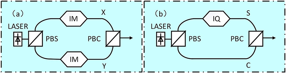
For SV-DD, the transmitted signal can be equivalently represented by a three-dimensional (3D) Stokes vector S=[S1,S2,S3]T, where T denotes the transpose of the vector. The Stokes vector can be defined as $$\begin{gathered} S0=|EX|2+|EY|2,S2=2Re{EX·EY*}, \\ S1=|EX|2−|EY|2,S3=2Im{EX·EY*}, \end{gathered}$$(1)where Re and Im stand for the real and imaginary part of a complex variable, respectively, and the asterisk superscript denotes the complex conjugate, while S0 is given by S0=S12+S22+S32. Here, for 2D transmission systems, we consider the two popular transmitters shown in Fig. 1. One of the transmitters, shown in Fig. 1(a), sends two intensity-modulated (IM) signals on an orthogonal SOP^[11]. The information of the signal is contained in the S0 and S1 components. Another transmitter, shown in Fig. 1(b), sends a complex signal (S) in X polarization, while a constant carrier (C) is sent in Y polarization^[12]. The signal information is contained in the S2 and S3 components.

Typical receivers of SV-DD are shown in Fig. 2. Receiver A, shown in Fig. 2(a), comprises a polarization beam splitter (PBS), two fiber optic couplers, a 90° optical hybrid, two balanced photodetectors (BPDs), and two PDs^[13]. The PBS splits the received signal into two orthogonal polarizations. Then, the two tributary signals are divided into four signals by the two 2×2 optical couplers; here, we assume that the 50/50 couplers are replaced by γ/(1−γ) couplers. After the 90° optical hybrid, we can detect the front-end output I=[I1,I2,I3,I4]T by the PDs. Vector [SR1,SR2,SR3]T can be straightforwardly acquired by receiver A. In order to further reduce cost, only two outputs of the 90° optical hybrid are detected by two PDs in receiver B, shown in Fig. 2(b), providing the outputs of |X+Y|2 and |X+iY|2. Components SR2 and SR3 cannot be obtained directly because only two outputs of a 90° optical hybrid are used. Figure 2(c) shows a novel Stokes vector receiver (SVR) with a 3×3 coupler^[10].

At the receiver, we can get the output currents of the photodetectors I=[I1,I2,I3,I4]+N, where N denotes the receiver noise. Here, we focus on the un-amplified system dominated by the thermal noise, assuming an additive Gaussian noise at the receiver N=[n1,n2,n3,n4]^[10,14]. The Stokes vector of the receiver SR can be obtained by SR=MI,(2)where M is the 4×4 mapping matrix given by M1=[11−γ0011−γ11−γ00−11−γ02γ00002γ0],M2=[11−γ0011−γ11−γ00−11−γ−11−γ4γ0−11−γ−11−γ04γ−11−γ],M3=[111121−γ−1−1−1−10−3γ03γ01γ−2γ1γ],(3)where M1, M2, and M3 are the mapping matrices of receivers A, B, and C, respectively. SR is obtained by using the front-end output I. The noise is mapped to the Stoke space as NS=MN. In Stokes space, the transfer equation can be written as SR=HST+NS,(4)where ST is the SV of the transmitter, NS is an additive noise vector, and H is the channel matrix. In this case, for simplicity, only a random polarization rotation is considered in the following theoretical derivations. Matrix H can be expressed by a Muller matrix H=[10000cos2ϕ−sin2ϕ00sin2ϕcos2ϕ00001],(5)where ϕ denotes the random polar angles. The Muller matrix H can be determined by pilot-aided or blind channel estimation^[15,16], and as the receiver has instantaneous knowledge of H, it reverses the channel effect to obtain S˜T=H−1HST+H−1NS=ST+N˜,(6)where S˜T is the approximate Stokes vector that we can calculate from output currents of the photodetectors, and noise vector N˜ undergoes the same transformation process, which can be expressed as N˜=H−1NS=H−1MN.(7)

As can be seen from Eq. (7), the receiver noise is changed with the mapping and channel estimation process when the data is recovered. Here, we use the SV-DD system with receiver A as an example to illustrate the variations of noise. By substituting H−1 and M1 into Eq. (7), N˜ can be written as N˜=H−1MN=[10000cos2ϕ−sin2ϕ00sin2ϕcos2ϕ00001]−1×[11−γ0011−γ11−γ00−11−γ02γ00002γ0]×[n1n2n3n4].(8)

It is apparent from Eq. (8) that the noise is related to the received ϕ of the SOP and the splitting ratio γ, where we omit the dispersion-related effects. For the PDM-IM systems, shown in Fig. 1(a), the intensity of the two polarizations is contained in ST0 and ST1. As can be seen from Eq. (6), S˜T0 and S˜T1 are related to n˜1 and n˜2, respectively. Therefore, n˜1 and n˜2 have an important effect on the PDM-IM system. The noise performance of the system can be demonstrated by a superposition of n˜1 and n˜2. Figure 3 shows the average noise power as a function of γ for different received SOPs. Noise power is normalized with respect to n1 and measured in decibels.

Here, we selected five SOPs (0°, 22.5°, 45°, 67.5°, and 90°), and demonstrated the effect of the splitting ratio, as shown in Fig. 3. It is apparent that the SOPs are symmetrically distributed around 45°; the curves of the 0° and 90° SOPs and the curves of the 22.5° and 67.5° SOPs are essentially the same. In addition, as shown in Fig. 3(a), the noise performance becomes completely independent from SOP for receiver A when γ=0.667 (SOP independent splitting ratio). For receiver B, the noise performance gradually approaches when γ>0.8. For receiver C, the noise performance becomes completely independent of the SOP when γ=0.5. Furthermore, when the SOPs are 0° and 90°, the noise performance is much better than that of other SOPs for receivers A and B. As can be seen from the polarization rotation matrix, S0 and S3 obviously do not vary with the SOP. Nevertheless, S1 and S2 can be transformed between each other by varying the SOP. When the SOPs are 0° and 90°, S˜T1 can be obtained by using SR1 only. When the SOP is 45°, S˜T1 is completely given by SR2, while in other cases, SR1 and SR2 need to be used. For the PDM-IM system, the intensity information is contained in S0 and S1; thus, SR0, SR1, and SR2 are necessary components. When γ is reduced below 2/3, more power is allocated to I1 and I4 in receivers A and B. As can be seen from Eq. (2) and M1, SR0 and SR1 are given by I1 and I4, respectively. This results in a much better performance when the SOP is close to 0° and 90°.

For the PDM-SC systems, shown in Fig. 1(b), the complex signal is contained in S2 and S3. Therefore, n˜3 and n˜4 have an important effect on the PDM-SC system. Figure 4 shows the average noise power as a function of γ for different received SOPs.

Like above, the noise performance is affected by the γ and the SOP. As shown in Figs. 4(a) and 4(c), the noise performance becomes completely independent of the SOP when γ=0.667 and γ=0.5. In contrast, the information of the PDM-SC signal is contained in S2 and S3; thus, the curve is apparently symmetric with respect to the curve in Fig. 3.

The simulation model for the proposed system is built by VPI transmission Maker 8.7 and MATLAB software. At the transmitter, as shown in Fig. 1, PAM4 and 16QAM signals are selected to simulate PDM-IM and PDM-SC systems, respectively. The transmission rate of the signal is set to 112 Gbit/s. Table 1 summarizes the general settings of the simulation parameters.

In addition to the parameters mentioned above, the shot noise is also considered in the simulation for the PDM-PAM4 system. The structure of the transmitter is shown in Fig. 1(a), and three receivers are shown in Fig. 2. It can be obviously seen in Figs. 5(a)–5(c) that the system performance is very close to the theoretical noise performance. The coupler splitting ratio and the SOP affect the system performance appropriately. The system performance becomes completely independent of the SOP when γ=0.667 and γ=0.5 for receivers A and C, respectively. For receiver B, the bit error rate (BER) performances converge to each other at γ=0.8. Figure 5(d) shows the back-to-back (BTB) BER as a function of received power for three SVRs, where all examined cases are plotted at the optimum coupler splitting ratio. The received optical power (ROP) of the three SVRs are −6.8dBm, −5.7dBm, and −8.4dBm at 7% forward error correction (FEC) threshold. Compared with receiver A, receiver C has a better ROP sensitivity by 1.6 dB.

For the PDM-SC-16-QAM system, the structure of the transmitter is shown in Fig. 1(b) and three receivers are shown in Fig. 2. The carrier-to-signal power ratio (CSPR) is 0 dB. The system performance becomes completely independent of the SOP when γ=0.667 and γ=0.5 for receiver A and receiver C, as shown in Fig. 6. For receiver B, it can be obviously seen that the optimal performance is achieved when γ=0.7. As shown in Fig. 7(d), the ROPs of the three SVRs are −8.7dBm, −6.6dBm, and −9.6dBm at 7% FEC threshold. Compared with receiver A, receiver C has a better ROP sensitivity by 0.9 dB.

In the previous simulation, we only considered the receiver noise, the coupler splitting ratio, and the SOP. Here, we present the results to further investigate the effect of EL on the system performance by simulation. The EL of the 90° hybrid is smaller than 2.5 dB, which is obtained by the datasheet of the commercial 90° hybrid (Kylia COH24). The EL of the 3×3 coupler is 0.15 dB, which is obtained by the datasheet of the commercial 3×3 coupler (Phoenix V1_0603). In this part of the simulation, we assume a 2.5 dB EL for the 90° hybrid and 0.15 dB EL for the 3×3 coupler.

Figures 7(a) and 7(b) show the BER performance as a function of the coupler splitting ratio with the 2.5 dB EL of the 90° hybrid. It can be obviously seen that the BER performance is independent of SOP when γ≈0.8 for both the PDM-IM and the PDM-SC systems using receiver A. The PDM-IM system using receiver A achieves a system BER below the 7% FEC threshold BER when γ=0.7, as shown in Fig. 7(a). We can conclude that 2.5 dB EL results in an ROP sensitivity penalty of ∼1.8dB. For the PDM-SC system, the optimum coupler splitting ratio is γ=0.8 and the 2.5 dB EL results in an ROP sensitivity penalty of ∼1.8dB. The input of the 90° hybrid requires more output to offset the power decline resulting from the EL. By selecting the appropriate optical coupler, the performance attenuation resulting from the EL can be reduced. For the 3×3 coupler-based SV-DD receivers, as shown in Figs. 7(c) and 7(d), the 0.15 dB EL results in an ROP sensitivity penalty of 0.25 dB for both the PDM-IM and the PDM-SC systems. The optimum coupler splitting ratio is maintained at γ=0.5. Table 2 summarizes and compares the 112 Gbit/s PDM-PAM4 and PDM-SC systems with different SV-DD receivers.

In this Letter, we studied the performances of the PDM-PAM4 and PDM-SC-16QAM signals using three different SV-DD receivers. In terms of system performance, the three crucial factors are the coupler splitting ratio, the SOP, and EL. In the 90° optical hybrid-based SV-DD receiver, the coupler with a 60/40 or 70/30 splitting ratio exhibits a better ROP performance than that with a splitting ratio of 50/50, especially for PDM-SC systems. It should be noted that the performance was completely independent of the SOP when a 67/33 coupler was used. Considering the 90° optical hybrid with a common EL of 2.5 dB, the 80/20 coupler achieved a steady performance independent of the SOP. In this case, there were receiver sensitivity penalties of 1.8 dB for both the PDM-IM and the PDM-SC systems. When 3×3 coupler-based SV-DD receivers were used, the best performance could be reached with a coupler splitting ratio of 50/50. Compared to receiver A, the PDM-IM and PDM-SC signals had better receiver sensitivities by 1.6 dB and 0.9 dB, respectively. Therefore, a cost-efficient 3×3 coupler-based SV-DD receiver is a promising choice for PDM-DD signals.

References

[1] L. Paraschis. European Conference and Exhibition on Optical Communication, Th.2.F.3(2013).