• Chinese Optics Letters
  • Vol. 20, Issue 4, 041101 (2022)
Weihao Wang1, Xing Zhao1、2、*, Zhixiang Jiang1, and Ya Wen1
Author Affiliations
  • 1Institute of Modern Optics, Nankai University, Tianjin 300350, China
  • 2Tianjin Key Laboratory of Optoelectronic Sensor and Sensing Network Technology, Tianjin 300350, China
  • show less
    DOI: 10.3788/COL202220.041101 Cite this Article Set citation alerts
    Weihao Wang, Xing Zhao, Zhixiang Jiang, Ya Wen. Deep learning-based scattering removal of light field imaging[J]. Chinese Optics Letters, 2022, 20(4): 041101 Copy Citation Text show less
    Overview of DeepSLFI. The light field imaging forward models can be built after the scattering imaging scene and the light field imaging system are determined. The simulation light field images serving as training samples can be generated with the forward models. Then, a neural network will be trained with the samples and utilized to remove the scattering of the light field image captured experimentally. Finally, the high-resolution and high-contrast 3D reconstruction can be obtained by 3D deconvolution with the deblurred light field image and the scattering-free forward model.
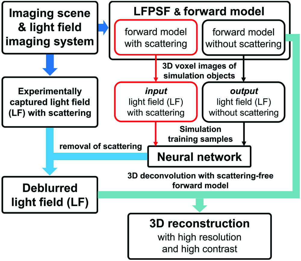
    Fig. 1. Overview of DeepSLFI. The light field imaging forward models can be built after the scattering imaging scene and the light field imaging system are determined. The simulation light field images serving as training samples can be generated with the forward models. Then, a neural network will be trained with the samples and utilized to remove the scattering of the light field image captured experimentally. Finally, the high-resolution and high-contrast 3D reconstruction can be obtained by 3D deconvolution with the deblurred light field image and the scattering-free forward model.
    Diagram of light field imaging forward model. Light emitted from voxels of object space g propagates to the sensor. The intensity distribution f on the sensor plane is the light field image. The column of H means light field point spread function (LFPSF), which is the proportion on the sensor of light emitted from the corresponding voxel of object space. With the f captured experimentally, g can be obtained by solving the inverse problem of the equation.
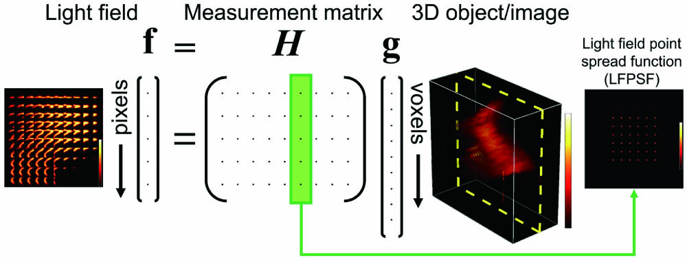
    Fig. 2. Diagram of light field imaging forward model. Light emitted from voxels of object space g propagates to the sensor. The intensity distribution f on the sensor plane is the light field image. The column of H means light field point spread function (LFPSF), which is the proportion on the sensor of light emitted from the corresponding voxel of object space. With the f captured experimentally, g can be obtained by solving the inverse problem of the equation.
    Light field images captured experimentally of the same object (a) without scattering and (b) with scattering. (a1) and (b1) correspond to the parts of the dashed boxes in (a) and (b), respectively. (c) The intensity curves of pixels on the blue and green lines.
    Fig. 3. Light field images captured experimentally of the same object (a) without scattering and (b) with scattering. (a1) and (b1) correspond to the parts of the dashed boxes in (a) and (b), respectively. (c) The intensity curves of pixels on the blue and green lines.
    Architecture of the neural network.
    Fig. 4. Architecture of the neural network.
    Diagram of the validation experimental system.
    Fig. 5. Diagram of the validation experimental system.
    Light propagation in the experimental system.
    Fig. 6. Light propagation in the experimental system.
    Generation process of the training samples.
    Fig. 7. Generation process of the training samples.
    Reconstruction results of the USAF target in the field of view. All of the images are scaled to [0,1]. (a) (i) Light field without scattering, (ii) with scattering, and (iii) deblurred by the network. (iv) The intensity curves of pixels corresponding to the lines in (i), (ii), and (iii). (v) The PSNRs and SSIMs of the LFs. (b) 3D reconstructions from perspective and orthogonal views (removed noise containing only several voxels that interferes with the observation), where the x and y directions are transverse directions, and the z direction is the depth/axial direction. The yellow dashed box shows the depth position of the object. (c) Slice images in the 3D reconstructions. (d) The intensity curves of voxels/pixels corresponding to the dashed lines in the slice images in (c), with (i) the curves of the manganese-purple dashed line in the x-y section, (ii) the curves of the green dashed line in the x-y section, (iii) the curves of the green dashed line in the x-z section, and also the manganese-purple dashed line in the y-z section. (iv) The PSNRs and SSIMs of the 3D reconstructions, where only the part consisting of areas in the yellow dashed box of each depth is selected for calculation. This is because the part outside is the edge of the field of view and has a low quality of reconstruction. It is not suitable for comparison of PSNRs and SSIMs affected by scattering.
    Fig. 8. Reconstruction results of the USAF target in the field of view. All of the images are scaled to [0,1]. (a) (i) Light field without scattering, (ii) with scattering, and (iii) deblurred by the network. (iv) The intensity curves of pixels corresponding to the lines in (i), (ii), and (iii). (v) The PSNRs and SSIMs of the LFs. (b) 3D reconstructions from perspective and orthogonal views (removed noise containing only several voxels that interferes with the observation), where the x and y directions are transverse directions, and the z direction is the depth/axial direction. The yellow dashed box shows the depth position of the object. (c) Slice images in the 3D reconstructions. (d) The intensity curves of voxels/pixels corresponding to the dashed lines in the slice images in (c), with (i) the curves of the manganese-purple dashed line in the x-y section, (ii) the curves of the green dashed line in the x-y section, (iii) the curves of the green dashed line in the x-z section, and also the manganese-purple dashed line in the y-z section. (iv) The PSNRs and SSIMs of the 3D reconstructions, where only the part consisting of areas in the yellow dashed box of each depth is selected for calculation. This is because the part outside is the edge of the field of view and has a low quality of reconstruction. It is not suitable for comparison of PSNRs and SSIMs affected by scattering.
    Results of reconstructions with different ways for two slits to be localized at different depths in object space. (a) The 3D reconstructions. The blue dashed boxes show the sizes and the positions of the slits. The “Depth” means the distance from the front plane of the depth of field. The median filtering is conducted at the edge of the lateral field of view to remove noise containing several voxels. (b) The PSNRs and SSIMs of the 3D reconstructions.
    Fig. 9. Results of reconstructions with different ways for two slits to be localized at different depths in object space. (a) The 3D reconstructions. The blue dashed boxes show the sizes and the positions of the slits. The “Depth” means the distance from the front plane of the depth of field. The median filtering is conducted at the edge of the lateral field of view to remove noise containing several voxels. (b) The PSNRs and SSIMs of the 3D reconstructions.
    Weihao Wang, Xing Zhao, Zhixiang Jiang, Ya Wen. Deep learning-based scattering removal of light field imaging[J]. Chinese Optics Letters, 2022, 20(4): 041101
    Download Citation