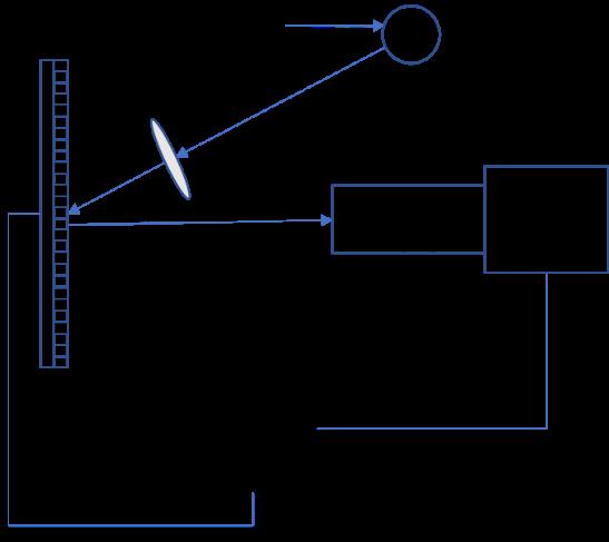
Fig. 1. Block compressed sensing（BCS）architecture with a graphics processing unit（GPU）acceleration imaging system

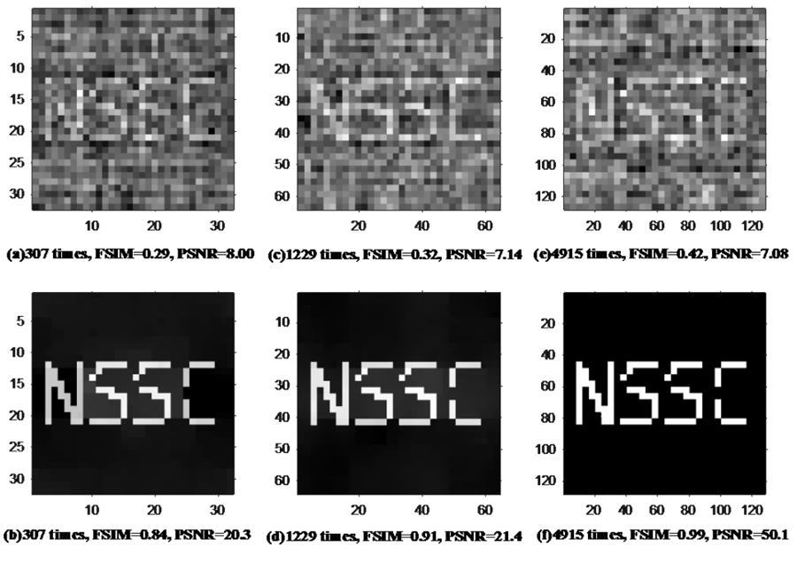
Fig. 2. Inverse（a，c，e）and CS（b，d，f）reconstruction results with subsampling rate = 0.3，the image sizes are（a），（b）32 × 32 pixels，（c），（d）64 × 64 pixels，and（e），（f）128 × 128 pixels

Fig. 3. Unit of projection vectors derived from a compressive element block. A part of the coding pattern on the SLM is divided into four identical parallelly measuring blocks. One measurement entry，which corresponds to a measurement operation and an observed value，is reshaped into a vector according to the vertical orientation

Fig. 4. Blocki is the observed value vector of the i-th compressed block used to recover the i-th original image block，Mj indicates the j-th measurement corresponding to j-th coding pattern，Blocki and Mj exactly indicate the observed value of i-th compressive block and j-th measurement，here，n=N×NC×C and m≤C×C

Fig. 5. Peak signal-to-noise ratio（PSNR）and reconstruction time with different block sizes and different under-sampling rates

Fig. 6. Block-compressive reconstruction procedure with GPU acceleration

Fig. 7. Comparison of experimental results from different low-resolution images with different compression ratios^［12］，a-1）–a-9）shows the digital chart，b-1）–b-9）is the film，c-1–c-9）is the toy，a，b，c-1），a，b，c-4）and a，b，c-7）are the low-resolution sampling images with 64 × 64 pixels，high-resolution MBCS reconstruction results with 128 × 128 pixels and the traditional block CS results，respectively，further，a，b，c-2），a，b，c-5）and a，b，c-8）are the low-resolution sampling images with 32 × 32 pixels，high-resolution MBCS reconstruction results with 128 × 128 pixels and the traditional block CS results，respectively，also，a，b，c-3），a，b，c-6）and a，b，c-9）are the low-resolution sampling images with 16 × 16 pixels，high-resolution MBCS reconstruction results with 128 × 128 pixels and the traditional block CS results，respectively

Fig. 8. Reconstruction time for the 128 × 128 scene by the MBCS algorithm using CPU and with GPU acceleration for different block sizes

Fig. 9. Reconstruction time for the 256 × 256 scene by the MBCS algorithm using CPU and with GPU acceleration for different block sizes

Fig. 10. Reconstruction time for the 512 × 512 scene by the MBCS algorithm using CPU and with GPU acceleration for different block sizes

Table 1. Comparison of the quality between traditional Block CS and MBCS

Table 2. Comparison of the reconstruction time between Matlab–CPU and GPU

Table 3. Comparsion of MBCS reconstruction times between the CPU algorithm and GPU acceleration for 128 × 128, 256 × 256, and 512 × 512 scenes. The first column lists the size of high-resolution images, HR stands for high resolution. The second column is the block size used to reconstruction, the third column shows the number of blocks in block reconstruction, the fourth column lists the time to recover one HR image in Matlab, the fifth column lists the time to recover one HR image by the MBCS algorithm with GPU acceleration, the sixth column lists the average time to recover each block of HR image, and it is equal to corresponding value in column “GPU (s)” divided by the corresponding value in column “Blks Cnt”