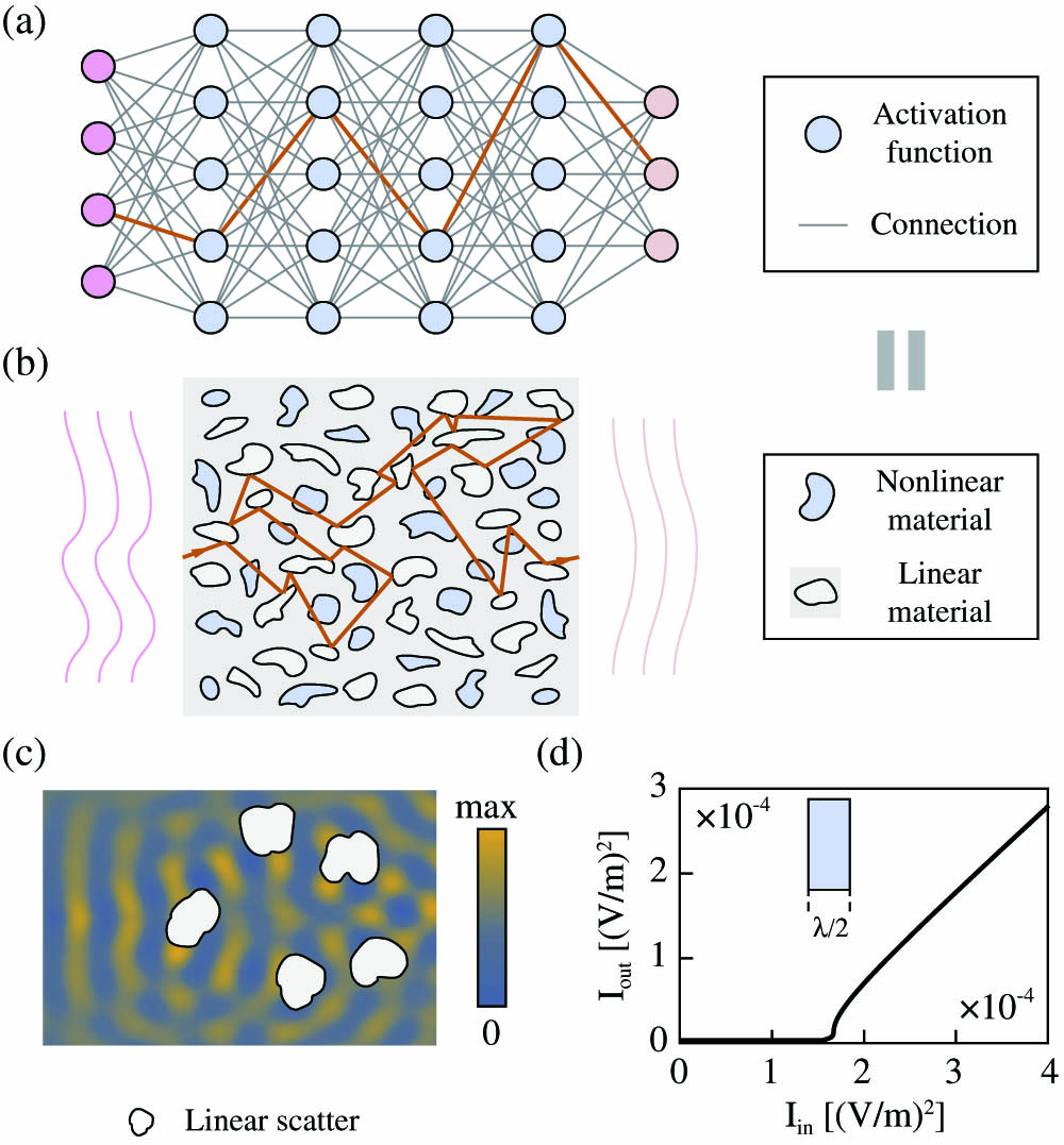
Fig. 1. (a) Conventional ANN architecture where the information propagates only in the forward direction (depicted by the green line that goes through the nodes from input to output); (b) proposed NNM. Passive neural computing is performed by light passing through the nanostructured medium with both linear and nonlinear scatterers. (c) Full-wave simulation of light scattered by nanostructures, which spatially redistribute the optical energy in different directions. (d) The behavior of the implementation of such a nonlinear material in one dimension. The output intensity of light with wavelength λ, passing through the designed nonlinear material with a thickness of λ/2. It is a nonlinear function of the incident wave intensity. This material is used as nonlinear activation, as indicated by light blue color.

Fig. 2. (a) NNM trained to recognize handwritten digits. The input wave encodes the image as the intensity distribution. On the right side of the NNM, the optical energy concentrates to different locations depending on the image’s classification labels. (b) Two samples of the digit 2 and their optical fields inside the NNM. As can be seen, although the field distributions differ for the images of the same digit, they are classified as the same digit. (c) The same as (b) but for two samples of the digit 8. Also, in both (b) and (c), the boundaries of the trained medium have been shown with black borderlines (see Visualization 1).

Fig. 3. (a) Training starts by encoding an image as a vector of current source densities in the FDFD simulation. This step is followed by an iterative process to solve for the electric field in a nonlinear medium. Next, we use the ASM to calculate the gradient, which is then used to update the level-set function and consequently, the medium itself. Here we use mini-batch SGD (explained in the supplementary materials section of Ref. [17]). In training with mini-batches, we sum the cost functions calculated for different images in the same batch and compute the gradients. (b)–(d) show an NNM in training after 1, 33, and 66 training iterations, respectively. (After iteration 66, the medium has already seen each of the training samples at least once, since we are using batches of 100 images.) At each step, the boundary between the host material and the inclusions is shown, along with the field distribution for the same randomly selected digit 8. Also, the accuracy of the medium on the test set can be seen for that particular stage in training.

Fig. 4. (a) 3D NNM case. Different colors illustrate varying values of permittivity. The input image is projected onto the top surface. Computing is performed while the wave propagates through the 3D medium. The field distribution on the bottom surface is used to recognize the image. Full-wave simulation shows the optical energy is concentrated on the location with the correct class label, in this case 6. (b) The confusion matrix. The rows on the matrix show true labels of the images that have been presented as input, and the columns depict the labels that the medium has classified each input. Therefore, the diagonal elements show the number of correct classifications out of every 10 samples (see Visualization 2).