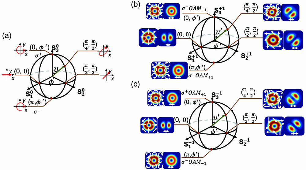
Fig. 1. (a) Polarization PS for representing the plane wave states of polarization. (b) The +1st-order PS and (c) the -1st-order PS. Modes and polarizations are provided for the states at the poles and for the special points on the equator.

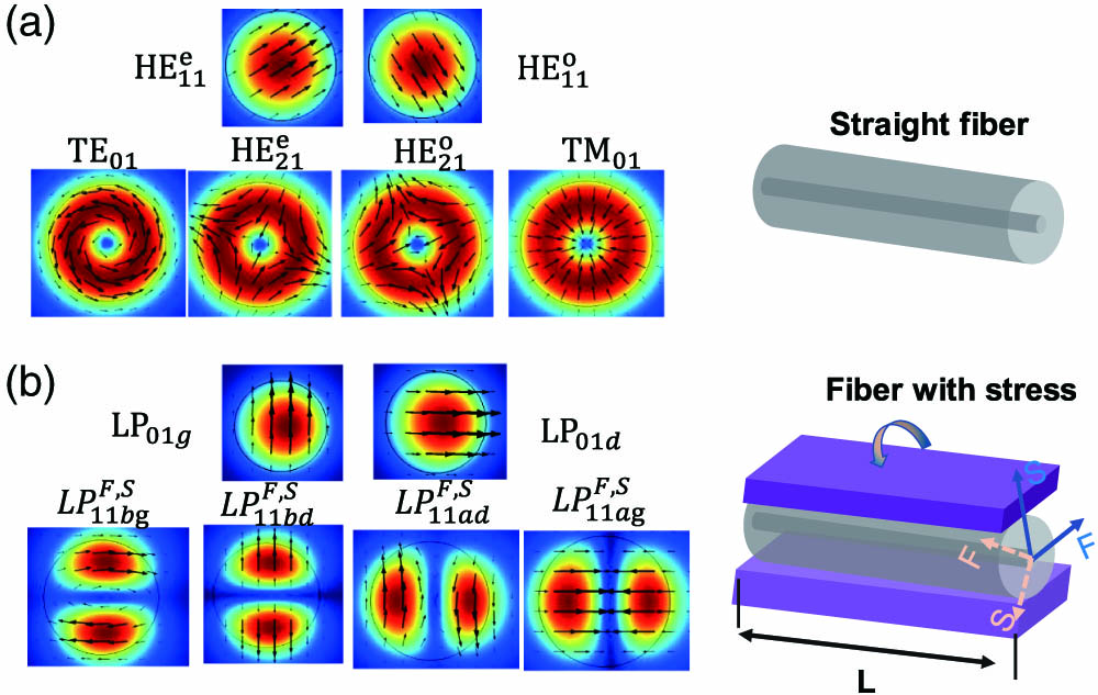
Fig. 2. (a) Eigenmodes in the FMF without stress. (b) Eigenmodes in the FMF with stress.

Fig. 3. (a) Schematic diagram to generate CV beams. (b) The polarizations and (c) modes along a longitude and a latitude on the two PSs. (b) and (c) show the mapping relationship between two PSs when the angle between g polarization and horizontal direction equals 0 deg.

Fig. 4. (a) Experimental setup to generate CV beams. Single-mode PC, single-mode polarization controller; PL, photonic lantern; Few-mode PC, few-mode polarization controller; Obj., objective; BS, beam splitter; QWP, quarter-wave plate; Pol., polarizer. (b) The microscope image of the few-mode-end cross section of the fabricated MSPL. (c) Near-field mode images at the few-mode end of the MSPL and output of 2 m FMF-tailed from the MSPL. (d) Phase differences between the four egienmodes varying the bending radius.

Fig. 5. (a) Experimental results and (b) simulation results when the input polarization is adjusted along the red line on the polarization PS, e.g., υ=π/2, and ϕ varies from 0 to 2π at intervals of π/4. (c) Experimental results and (d) simulation results when the input polarization is adjusted along blue line with ϕ=π/2 and υ varying from π to −π at intervals of π/4.

Fig. 6. Correlation coefficients for the modes of I(0°,0°),I(90°,90°),I(45°,45°), and I(135°,135°). (a) When υ=π/2, and ϕ at intervals of π/4; (b) when ϕ=π/2 and υ varies from −7π/4 to π at intervals of π/4.

Fig. 7. Polarization distributions of the modes along the longitude and latitude on the FOPS.

Fig. 8. Detailed comparison between our approach and others’. The yellow rows represent the free-space system, and the green rows represent the all-fiber system.