Fig. 1. Diagram of the focusing system (microscope objective) illustrating the reference coordinate systems and the variables involved in the process [44].

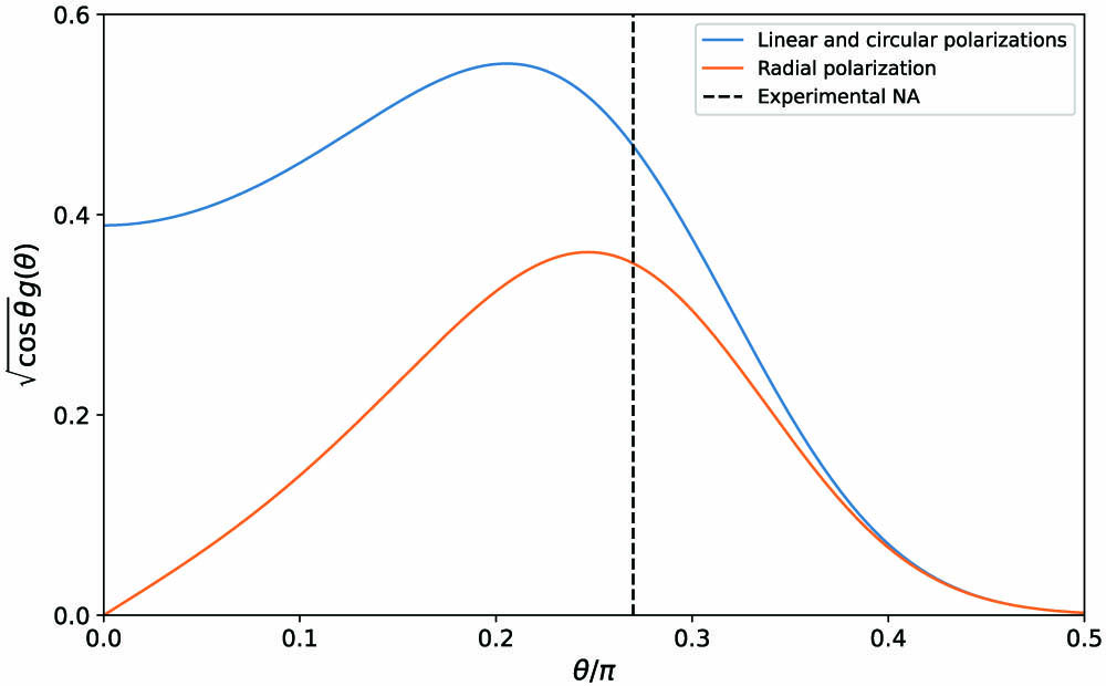
Fig. 2. Blue and orange solid lines represent the field amplitudes in, respectively, Eqs. (14) and (16) multiplied by the prefactor cos θ, as it appears in Eq. (11). The vertical dashed line denotes the angular value associated with the numerical aperture considered here.

Fig. 3. Bloch sphere diagram illustrating the state of homogeneous polarization u^X [Eq. (15)]. Along the different axes are the six more representative elements of the three usual two-vector basis sets: {u^H,u^V}, {u^D,u^A}, and {u^R,u^L}.

Fig. 4. (a) Representation of the Di functions in Eq. (21), in terms of the radial distance r for g(θ) given by Eq. (14). D0 is denoted with a solid blue line, D1 with the dashed orange line, and D2 with the dash-dotted green line. (b) Representation of the Di′ functions in Eq. (37), in terms of the radial distance r, for g(θ) given by Eq. (16). The solid blue line and the dashed orange line denote, respectively, D0′ and D1′.

Fig. 5. Vector plots of the normal direction vector N(X)(r,ϕ) at the focal plane (z=0) for input fields with different polarization states. (a) Linear (horizontal) polarization in Eq. (24). (b) Radial polarization in Eq. (40). (c) and (d) Circular right-handed polarization in Eq. (33). A 3D picture is represented in panel (c), while panel (d) offers a 2D representation with only the transverse components of N(c)(r,ϕ). In panels (a), (b), and (d) a density plot of the irradiance at the focal plane is also provided to have an idea of the spatial region where the field energy is mainly concentrated. The color scale, from black to light green, indicates the increasing value of the irradiance. In these calculations, σ=2 and NA=0.75, as in the experiments.

Fig. 6. Experimental value obtained for the transverse Stokes parameters (top row) and local Stokes parameters (middle row) at the focal plane for a linearly polarized input field, with horizontal polarization. The local Stokes parameters obtained numerically are shown in the bottom row of the figure for comparison. The color code on the right-hand side applies to all the panels. The input beam has been produced with σ=2 and the focusing optical system has NA=0.75.

Fig. 7. Experimental value obtained for the transverse Stokes parameters (top row) and local Stokes parameters (middle row) at the focal plane for a circularly polarized input field, with right-handed polarization (γ=+1). The local Stokes parameters obtained numerically are shown in the bottom row of the figure for comparison. The color code on the right-hand side applies to all the panels. The input beam has been produced with σ=2 and the focusing optical system has NA=0.75.

Fig. 8. Experimental value obtained for the transverse Stokes parameters (top row) and local Stokes parameters (middle row) at the focal plane for a radially polarized input field. The local Stokes parameters obtained numerically are shown in the bottom row of the figure for comparison. The color code on the right-hand side applies to all the panels. The input beam has been produced with σ=2 and the focusing optical system has NA=0.75.

Fig. 9. Experimental setup (see the main text for details). To produce a linearly polarized input field, QWP2 is removed, while it is replaced by the VR if radially, azimuthally, or spirally polarized input fields are required.

Fig. 10. Experimental data management pipeline. See the main text for a detailed explanation of each processing block. FFSP, forward free space propagation; BFSP, backward free space propagation; h(·), the convolution kernel of the Fresnel diffraction; and *, the convolution product.