Fig. 1. Coupled-waveguides system with its representation of the complex eigenvalues as Riemannian surfaces. (a) Two coupled waveguides, as lossless and lossy ones, respectively, form an integrated system that possesses a Hamiltonian H0. (b), (c) Riemannian surfaces of the complex eigenvalues [real (b) and imaginary (c) parts] of the matrix H0 versus the (κ0,γ0) parameters, where the blue regions represent PT-broken and red ones are PT-symmetric regions. In addition, the boundary is considered as lines of EPs. Notably, these Riemannian surfaces contain the PT-symmetric coupled subsystem and decaying subsystem for a realistic manifestation. The existence of a decaying subsystem causes a tilt angle for the surface in (c).

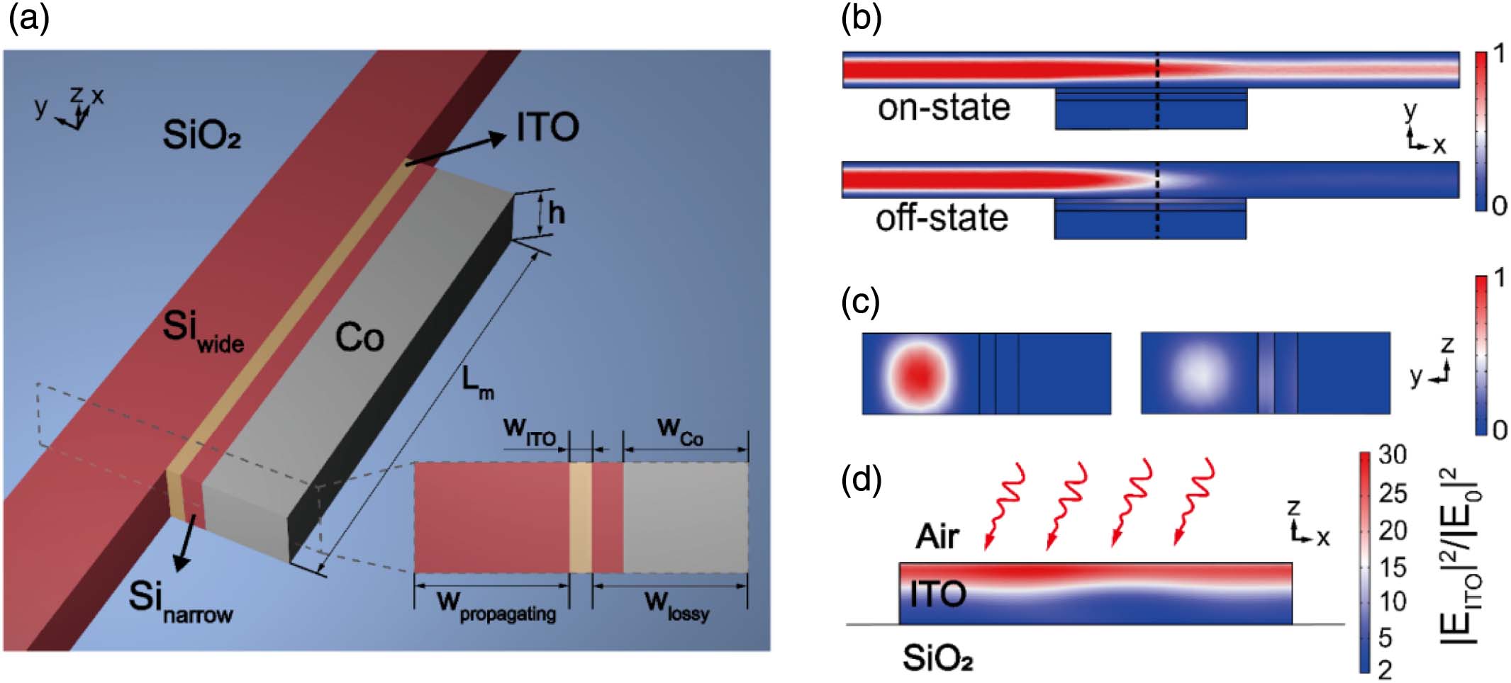
Fig. 2. Schematics of the proposed modulator, internal electric-field, and power-flow distribution. (a) Structure of modulator integrated on SiO2 (blue) substrate. ITO (yellow) is sandwiched between the propagating waveguide composed of Siwide and hybrid lossy waveguide composed of Sinarrow and cobalt (gray). Note that both red regions represent silicon. Inset shows the cross-section at the yz plane. Widths of propagating and hybrid lossy waveguides are set to be the same, namely, Wpropagrating=Wlossy=280  nm. Besides, WITO=40  nm and WCo=224  nm are the width of ITO and cobalt, respectively. Furthermore, ITO and two waveguides are designed with the same height h=200  nm. Last, the modulation length is considered to be within one wavelength, Lm=1240  nm. (b), (c) Power-flow in the modulator at on-state and off-state from xy plane and yz plane views. The black dashed lines in (b) mark the location of the yz-plane view in (c), where the coupled energy in hybrid lossy waveguide reaches the maximum. (d) Field enhancement at the central cross-section at xy plane in ITO. Pump laser (1250 nm, 30° incident angle) marked as red spiral curves is imposed on ITO. EITO means the electric field at ITO and E0 is the incident electric field.

Fig. 3. Analysis of PT-symmetric and PT-broken regions and eigenvalue spectra of the whole modulator system. (a) Transmitted power efficiency varies with WCo from 14 to 280 nm. The blue dashed and solid curves mean systems with and without pump, respectively. The red curve represents the calculated extinction ratio. (b) The calculated coupling coefficients κ with pump (blue dashed curve) and without pump (blue solid curve). The range of WCo is captured from 112 to 266 nm to study the change of κ around EP. The red curve presents the ratio of coefficients with and without pump. (c), (d) The WCo dependent κ (black curve) and the propagation loss of hybrid waveguide γ2 (blue curve) (c) without pump and (d) with pump. The red curve that represents |γ1−γ2|/2 is designed to compare with κ to judge whether the system is in the status of PT-symmetric (blue regions) or PT-broken (gray regions). (e), (f) The relative-loss γ=|γ1−γ2| dependent eigenvalue spectra of the system. Four legends with different colors mark the eigenvalues with and without pump. Due to the fluctuation of coupling coefficient, the spectra are not smooth as expected.

Fig. 4. Analysis of the balance between extinction ratio and on-state transmitted efficiency. (a), (b) The WCo-dependent extinction ratio and on-state transmitted efficiency under different WITO from 30 to 70 nm. Note that the legends are the same for both (a) and (b). (c), (d) Two ultimate states of power-flow distribution at the xy plane where WITO is 30 nm in (c) and 70 nm in (d).

Fig. 5. Electric-field distribution of the input port for propagating waveguide.

Fig. 6. Transmitted efficiency versus pump intensity.

Fig. 7. Normalized electric-field distributions in the hybrid lossy waveguide. (a) Schematic of the whole system at the xy plane. Hybrid lossy waveguide composed of Sinarrow and cobalt is marked as the gray dashed rectangle; width of cobalt is marked as WCo. (b)–(i) Electric-field distributions in hybrid lossy waveguide under different WCo, which is from 40 to 250 nm (as the example when ITO is under pump). Note that the electric field is mainly distributed in Sinarrow and sorted into two parts, E1 and E2, which are marked as the black and white circles, respectively, in (b).

Fig. 8. Normalized transmitted power in hybrid lossy waveguide that is used for calculation of coupling coefficients. (a) Schematic of the simulation structure. The red cross section in hybrid lossy waveguide is used to calculate the surface integral of power flow at each location. (b), (c) Situations without and with pump, respectively. The x-label is the transmitted distance, and each curve means the situation for the specified width of cobalt (from 28 to 252 nm). The coupling length is exactly the distance where the transmitted power reaches the maximum.

Fig. 9. Simulation structures for the calculation of propagation loss and their normalized transmitted power (as the example when ITO is under pump). (a) The propagating waveguide with a half of ITO. (b) The hybrid lossy waveguide with a half of ITO. The imaginary part of the refractive index in the left part (marked as lossless part by gray dashed rectangle) is deliberately set to be zero for the more realistic simulation of the propagating and coupling mechanism, which leads to a sharp decay when light propagates to hybrid lossy waveguide. (c), (d) The decay curves of the transmitted power in (a) and (b). The initial positions (x=0) are where the propagating waveguide has ITO for (c) or at the interface of the lossless part and hybrid lossy waveguide for (d). Note that curves in (d) are presented under different widths of cobalt (from 28 to 252 nm).

Fig. 10. Calculation for propagation speed, which is the ratio of the apparent change in ω to the associated change in β.