
Xiujia Dong, Yao Ding, Zhengyang Bai, Guoxiang Huang. Magnetic-field-induced deflection of nonlocal light bullets in a Rydberg atomic gas[J]. Chinese Optics Letters, 2022, 20(4): 041902
- Chinese Optics Letters
- Vol. 20, Issue 4, 041902 (2022)
![(a) Excitation scheme of the Rydberg EIT. |1〉, |2〉, and |3〉 are, respectively, the ground, intermediate, and Rydberg states; Ωp (Ωc) is the half-Rabi frequency of the probe (control) laser field; Γ12 (∼MHz) and Γ23 (∼kHz) are, respectively, decay rates from |2〉 to |1〉 and |3〉 to |2〉; Δ2 = ωp − (ω2 − ω1) and Δ3 = ωp + ωc − (ωc − ω1) are, respectively, the one- and two-photon detunings. ℏV(r − r′) is the vdW interaction between the two atoms in Rydberg states, respectively, located at r and r′. (b) Geometry of the system. The probe and control fields counter-propagate in the Rydberg atomic gas. (c) Normalized χp,2(3) (i.e., the coefficient of nonlocal Kerr nonlinearity) as a function of coordinate x, with the solid black (dashed red) line representing its real part Re(χp,2(3)) [imaginary part Im(χp,2(3))] for coordinate y = 0 (see text for more details). Evolution of a (d1) nonlocal LB and (d2) vortex in the system.](/richHtml/col/2022/20/4/041902/img_001.jpg)
Fig. 1. (a) Excitation scheme of the Rydberg EIT. |1〉, |2〉, and |3〉 are, respectively, the ground, intermediate, and Rydberg states; Ωp (Ωc) is the half-Rabi frequency of the probe (control) laser field; Γ12 (∼MHz) and Γ23 (∼kHz) are, respectively, decay rates from |2〉 to |1〉 and |3〉 to |2〉; Δ2 = ωp − (ω2 − ω1) and Δ3 = ωp + ωc − (ωc − ω1) are, respectively, the one- and two-photon detunings. ℏV(r − r ′) is the vdW interaction between the two atoms in Rydberg states, respectively, located at r and r ′. (b) Geometry of the system. The probe and control fields counter-propagate in the Rydberg atomic gas. (c) Normalized χp,2(3) (i.e., the coefficient of nonlocal Kerr nonlinearity) as a function of coordinate x, with the solid black (dashed red) line representing its real part Re(χp,2(3)) [imaginary part Im(χp,2(3))] for coordinate y = 0 (see text for more details). Evolution of a (d1) nonlocal LB and (d2) vortex in the system.
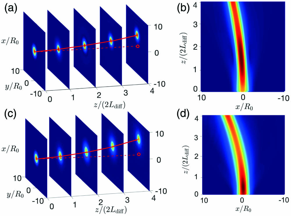
Fig. 2. Stern–Gerlach deflections of nonlocal LBs. (a) 3D motion trajectory of an LB as a function of x/R0, y/R0, and z/(2Ldiff) in the presence of the gradient magnetic field (B1,B2) = (3.2, 0) mG cm−1; (c) 3D motion trajectory of the LB for (B1, B2) = (6.4, 0) mG cm−1. (b) and (d) are trajectories of the LB in the x–z plane, corresponding, respectively, to panels (a) and (c).
Fig. 3. Motion trajectory of the LB in the presence of a time-varying gradient magnetic field. (a) Trajectory of the LB as a function of x/R0, y/R0, and z/(2Ldiff) when the time-varying gradient magnetic field of Eq. (9 ) is present. (b) The corresponding sinusoidal trajectory of the LB in the x–z plane.

Set citation alerts for the article
Please enter your email address
© Copyright 2018-2021 | Chinese Laser Press. All Rights Reserved 沪ICP备15018463号-20