
[in Chinese], [in Chinese], [in Chinese], [in Chinese], [in Chinese]. Underwater image enhancement based on red channel weighted compensation and gamma correction model[J]. Opto-Electronic Advances, 2018, 1(10): 180024
- Opto-Electronic Advances
- Vol. 1, Issue 10, 180024 (2018)
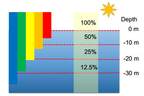
Fig. 1. Light absorption at different wavelengths underwater.
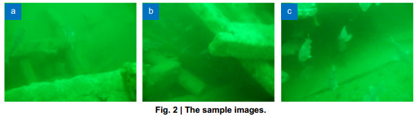
Fig. 2. The sample images.
Fig. 3. RGB channels and corresponding histogram distribution . (a ) Original image. (b ) R channel. (c ) G channel. (d ) B channel. (e ) Histogram distribution of R. (f ) Histogram distribution of G. (g ) Histogram distribution of B.
Fig. 4. (a ) Underwater image. (b ) Estimated theoretical value in red rectangle. (c ) RGB color cube.
Fig. 5. (a ) Original image. (b ) Red channel after compensation. (c ) Red channel after guided filtering. (d ) New RGB image.
Fig. 6. (a ) Histogram. (b ) Cumulative histogram.
Fig. 7. Gamma correction curve.
Fig. 8. Algorithm flow . (a ) Original image. (b ) After compensation. (c ) γ =0.8.
Fig. 9. (a ) Original image. (b ) γ =0.3. (c ) γ =0.6. (d ) γ =0.9. (e ) γ =1.2. (f ) γ =1.5.
Fig. 10. Comparison of different methods . (a ) Original images. (b ) DCP. (c ) Histogram equalization. (d ) Gray World. (e ) UCM. (f ) Our results.
Fig. 11. Comparison of different methods of actual underwater images . (a ) Original images. (b ) Histogram equalization. (c ) UDCP. (d ) Gray World. (e ) UCM. (f ) Our result.
Fig. 12. Video restoration by proposed algorithm.
|
Table 1. The entropy of images.
|
Table 2. The contrast of images.
| ||||||||||||||||||||||
Table 3. Calculation time for different resolutions.


Set citation alerts for the article
Please enter your email address

© Copyright 2018-2021 | Chinese Laser Press. All Rights Reserved 沪ICP备15018463号-20