The ocean contains a large amount of resources, and the video acquired by underwater imaging equipment is essential when exploring marine resources¹. In recent years, more and more underwater robot equipments have been put into applications. Underwater resource exploration, underwater facilities maintenance, and submarine tourism require a large amount of underwater data². Due to the special optical environment in ocean, the acquired video is prone to suffer from quality degradation such as color shift, edge blur and contrast reduction³. Degraded images cause huge trouble for subsequent research work⁴. Therefore, underwater imaging has received much attention and many scholars have done a lot of researches⁵.

The current improvement methods of underwater images mainly fall into two categories⁶: One category is based on traditional underwater image enhancement algorithms such as histogram equation⁷, wavelet transform⁸, sharpening⁹ and Retinex¹⁰ etc. They do not consider the principle of underwater imaging, but mainly optimize the color or contrast by adjusting the pixel values. In 2007, Iqbal et al.¹¹ proposed an underwater image enhancement algorithm using an integrated color model (ICM) based on sliding histogram, which successively stretched in RGB and HSI color gamut to enhance the image. But the algorithm needs to manually adjust the parameters according to the input image. In 2010, Iqbal et al.¹² proposed an unsupervised color correction method (UCM) based on Von Kries hypothesis (VKH) and selective histogram stretching. The UCM algorithm can effectively improve the brightness, but the restored image still shows chromaticity unevenness. In 2015, Ghani et al.¹³ used the Rayleigh distribution function to redistribute the original image based on Iqbal's work. This algorithm can improve the contrast of the image, but it is easy to introduce noise and reduce the signal-to-noise ratio. The other category is based on image restoration algorithm which establishes scattering model to reconstruct clear image. Zhao et al.¹⁴ modeled the background light of the scattering model to provide optimized parameter design for underwater imaging system under natural light and artificial lighting conditions. But the experimental results under this model had not been given by the authors. Since the underwater environmental model is similar to the natural outdoor imaging model, many researchers applied the Dark Channel Prior (DCP) dehazing algorithm proposed by He et al.¹⁵ to underwater image restoration. Li et al.¹⁶ used the guided triangular bilateral filtering based on the DCP algorithm to restored underwater image. But the image is overall dark after processing with this algorithm. Yang et al.¹⁷ proposed to use minimum and medium filtering instead of soft matting to reduce computational complexity based on DCP. This algorithm uses color correction to improve the contrast, but low quality restoration results limit the visual effect of the output image. Drews et al.¹⁸ proposed an underwater DCP (UDCP) algorithm based on blue-green channel to estimate more accurate transmission map. But the restored image is prone to brightness saturation. Image restoration based on dehazing model is often accompanied with complex calculation which is not suitable for real-time video system.

Take typical image taken at a depth of about 10 m in the Bohai Sea by Yantai Institute of Coastal Zone Research, Chinese Academy of Sciences as an example, the red component in the image is attenuated sharply. The blue-green background dominates the whole image. And the captured image is blurred. For images in similar scenes, we tested a variety of existing underwater enhancement and restoration algorithm. But the results after processing are not satisfactory. It is still challenging to restore images with red component attenuation. In this paper, a new underwater enhancement algorithm for similar complex scenes is proposed without estimating complex water parameters. The following arrangements are as follows: At first, we analyze the characteristics of typical ocean image attenuation and describe problems pertaining to underwater images. Then the enhancement model and algorithm are introduced in detail. Next we compare the experimental results with other literatures and conclude this paper in the end.

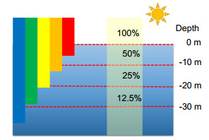
Water absorbs light with longer wavelength significantly. Most of the red light can only penetrate 2-3 m¹⁹. The light of different wavelengths decays with depth in water as shown in Fig. 1. In addition, underwater imaging is also affected by other factors such as distance, turbidity of water and illumination. The attenuation of underwater light during propagation is consistent with Lambert-Beer law²⁰. The law states that the attenuation of light in the medium is exponentially related to the transmission distance, as shown in equation (1):

where β_λ is a transmission factor related to wavelength λ. d(x) is the transmission distance. And t_λ(x) is the transfer function of light.

The typical images collected about 10 m deep in the Bohai Sea are shown in Fig. 2. Obviously, the green color dominates the whole image.

As shown in Fig. 3, we separate the RGB channels and calculate the data distribution in different channels. The grayscale values in the red channel are basically distributed in the extreme left side of the histogram. The edge features in the red channel are seriously lost, which results in uneven color distribution in RGB image. The channel with missing information is a great obstacle to the subsequent image restoration. Therefore, it is very meaningful to propose an algorithm to estimate the pixel intensity and edge information in the red channel.

In RGB color space, different ratios of the three primary colors can produce various intermediate colors, such as white when the values of three primary colors are [255, 255, 255]. If the images are captured in outdoor conditions, the color of the sky background or artificial lighting area should tend to be at the vertex of the RGB color cube, as shown in Fig. 4. In theory, the pixel value in the red rectangle in Fig. 4(a) should approach the value in Fig. 4(b). The absence of red channel's information in Fig. 4(a) causes the background to be blue-green.

The Gray World²¹ algorithm considers that for an image with large numbers of color changes, the average value of RGB channels tends to the same gray value. Similarly, when a natural image in outdoor condition is separated into RGB channels, it can be found that the separated three images are similar in the edge. In DCP algorithm, the guided image is selected as any of the separated RGB images when using guided filtering²² to refine the transmission map. The typical images collected in Bohai Sea are mainly attenuated in red channel. The intensity and edge information are almost completely missing in red channel while the blue and green channels still retains the edge features. So we consider using the information of other channels to compensate the red channel.

The experiment results²³ show that there is an approximate linear relationship between the underwater scattering coefficient b_λ and the wavelength λ. They derived this inference by analyzing the data of nine wavelengths collected in different waters using least squares regression analysis. This inference was widely quote by later scholars. It can be formulated as follows:

2 $ {{b}_{\lambda }}=(-0.00113\lambda +1.62517)b({{\lambda }_{\text{r}}})\;\;, $

where λ_r is the reference wavelength depending on the property of the measuring device (i.e. 555-nm for an AC9 meter in Ref. ²³). In this paper, we only consider the proportional relationship of the scattering coefficient of different wavelengths, so b(λ_r) does not need to be obtained by additional means in advance. We select the wavelength of red, green and blue to be 620 nm, 540 nm and 450 nm.

The attenuation coefficient c_λ for different wavelength λ is inversely proportional to its corresponding background light B_λ, and is proportional to the scattering coefficient b_λ²⁴. So the ratios of attenuation coefficient between three channels can be calculated as follows:

3 $ \frac{{{c}_{\text{g}}}}{{{c}_{\text{r}}}}=\frac{{{b}_{\text{g}}}{{B}_{\text{r}, \infty }}}{{{b}_{\text{r}}}{{B}_{\text{g}, \infty }}}\ \ , $

4 $ \frac{{{c}_{\text{b}}}}{{{c}_{\text{r}}}}=\frac{{{b}_{\text{b}}}{{B}_{\text{r}, \infty }}}{{{b}_{\text{r}}}{{B}_{\text{b}, \infty }}}\ \ , $

where B_{λ, ∞} is the background light at infinity. We take the brightest 0.1% pixels in each channel as the background light in this paper.

The attenuation of the underwater image remains approximately unchanged in a local region. So median filtering is adopted to keep the local intensity information of each channel. Define the three channels after filtering as R_med, G_med and B_med:

5 $ {{R}_{\text{med}}}={{f}_{\text{medfilt}}}(R)\ \ , $

6 $ {{G}_{\text{med}}}={{f}_{\text{medfilt}}}(G)\ \ , $

7 $ {{B}_{\text{med}}}={{f}_{\text{medfilt}}}(B)\ \ , $

where f_medfilt is the median filtering operation on each channel. The size of filtering widow is defined as 15×15.

We know that the attenuation in red channel is strong while the attenuation in green and blue channels is weak, so we compensate the intensity information of red channel based on the other two channels. Define the compensation coefficients of three channels as ω_r, ω_g and ω_b. According to the attenuation ratio, the compensation coefficients are normalized to:

8 $ {{\omega }_{\text{r}}}={{(1+\frac{{{c}_{\text{g}}}}{{{c}_{\text{r}}}}+\frac{{{c}_{\text{b}}}}{{{c}_{\text{r}}}})}^{-1}}\ \ , $

9 $ {\omega _{\rm{g}}} = \frac{{{c_{\rm{g}}}}}{{{c_{\rm{r}}}}} \cdot {(1 + \frac{{{c_{\rm{g}}}}}{{{c_{\rm{r}}}}} + \frac{{{c_{\rm{b}}}}}{{{c_{\rm{r}}}}})^{ - 1}}\;\;, $

10 $ {\omega _{\rm{b}}} = \frac{{{c_{\rm{b}}}}}{{{c_{\rm{r}}}}} \cdot {(1 + \frac{{{c_{\rm{g}}}}}{{{c_{\rm{r}}}}} + \frac{{{c_{\rm{b}}}}}{{{c_{\rm{r}}}}})^{ - 1}}\;\;, $

Then the red channel after weighted compensation can be calculated as:

11 $ {R_{{\rm{new}}}} = {\omega _{\rm{r}}} \times R + {\omega _{\rm{g}}} \times G + {\omega _{\rm{b}}} \times B\;\;, $

As shown in equation (11), if the intensity and edge information has been attenuated to a very low level, the information in the red channel can be compensated in this way. Note that the edge information is blurred after median filtering, so guided filtering²² is applied to refine the compensated red channel. The guided filtering filters the target image q through a guided image I, making the final output image similar to the target image q in intensity, but the edge similar to the guided image I. The output image q and the guided image I can be represented by the following local linear model:

12 $ {q_i} = {a_k} \cdot {I_i} + {b_k}, \forall i \in {\omega _k}\;\;, $

where i, k is the pixel index, and a, b is the coefficient of the linear model when the window located at k.

Since the green channel is rich in edge, we use green channel as the guided image to refine the compensated red channel R_new to obtain the final output red channel R_new^GF. Finally, the compensated red channel and the green, blue channel are combined into a new RGB image. The flow of red channel weighted compensation is shown in Fig. 5. Figure 5(a) is the original image. Figure 5(b) is the red channel after local intensity compensation. Figure 5(c) is the red channel after guided filtering on Fig. 5(b), and Fig. 5(d) is the final compensated image. It is obvious that the red channel is compensated and the background is bright and natural.

After compensating the background color in the previous part, the resulting image temporarily retains low contrast and poor visual effect which is not satisfactory enough. So in this part, we use a method based on grayscale stretching to improve the contrast of the image.

Firstly, we calculate the histogram distribution of three channels on the compensated image as shown in Fig. 6(a). Then the cumulative histogram can be calculated according to the histogram, so that the cumulative proportion is sorted by intensity as shown in Fig. 6(b). The gamma correction is based on the whole intensity distribution of the image. Considering the extreme points in the image such as noise caused by the environmental conditions or the imaging sensors, we search the maximum and minimum values in the original image by means of range search. Based on the previous data analysis, the grayscale value of the three channels is only distributed in a partial range. We define the minimum value before stretching as I_low and search for I_low as follows:

13 $ {I_{{\rm{low}}}} = \{ i|\min (\sum\nolimits_{j = 0}^i {hist(j)} \ge {r_1}), \;0 \le i \le 255\} \;\;, $

where $ \sum\nolimits_{j = 0}^i {hist(j)} $ is the proportion of pixels whose intensity is less than or equal to i, and r₁ is the pre-set value.

Similarly, we define the maximum value before stretching as I_high and search for I_high as follows:

14 $ {I_{{\rm{high}}}} = \{ i|\min (\sum\nolimits_{j = 0}^i {hist(j)} \ge {r_2}), \;0 \le i \le 255\} \;\;, $

where r₂=1-r₁.

The process of selecting the stretching interval [I_low, I_high] in the cumulative histogram is shown in Fig. 6. In order to facilitate the reader's viewing, we set r₁=0.1 in Fig. 6(b). Then its corresponding abscissa is the selected I_low. I_high can be obtained in the same way.

We define the range after stretching as [O_low, I_high]. Theoretically, the image gets the maximum contrast when the range is [0, 255] after stretching. We use the following gamma correction formula to do the stretching.

15 $ O(x) = \left\{ {\begin{array}{*{20}{c}} {{O_{{\rm{low}}}}\;\;\;\;\;\;\;\;\;\;\;\;\;\;\;\;\;\;\;\;\;\;\;\;\;\;\;\;\;\;\;\;\;{\rm{, }}I(x) \le {I_{{\rm{low}}}}}\\ {{O_{{\rm{low}}}} + ({O_{{\rm{high}}}} - {O_{{\rm{low}}}}) \times {{(\frac{{I(x) - {I_{{\rm{low}}}}}}{{{I_{{\rm{high}}}} - {I_{{\rm{low}}}}}})}^\gamma }\;{\rm{, }}{I_{{\rm{low}}}} < I(x) \le {I_{{\rm{high}}}}}\\ {{O_{{\rm{high}}}}\;\;\;\;\;\;\;\;\;\;\;\;\;\;\;\;\;\;\;\;\;\;\;\;\;\;\;\;\;\;\;\;\;\;\;{\rm{, }}{I_{{\rm{high}}}} < I(x)} \end{array}} \right.. $

In the original image, the pixel whose grayscale value is less than I_low is assigned to O_low in the output image. The pixel whose grayscale value is greater than I_high is assigned to O_high. For the correction parameter γ, the range close to I_low is stretched and the range close to I_high is compressed if γ < 1, the image will become brighter. On the contrary, if γ > 1, the image will become darker. The gamma correction model is shown in Fig. 7.

The process of image after weighted compensation and gamma correction is shown in Fig. 8. The image shown in Fig. 8(c) is the result when r₁=0.01, r₂=0.99 and γ= 0.8. The contrast is significantly improved on the basis of weighted compensation. For typical image collected in Bohai Sea, the restoration results are shown in Fig. 9 when γ ranges from 0.3 to 1.5. When γ= 0.3, the overall brightness is enhanced and the upper part of the image is supersaturated. As γ increases, the brightness of image gradually decreases. It is obvious that the restored image has a more natural visual effect.

Another advantage of this algorithm is that the transition between bright area and other areas is smooth which can prevent distortion from external lighting sources. More experimental results are shown in the next section.

The experimental video is captured with a GoPro camera at a depth of about 10 m in the Bohai Sea by Yantai Institute of Coastal Zone Research. The experiment hardware platform is a desktop with Inter(R) Core(TM) i5-6500 CPU@3.20 GHz, 16G RAM and NVDIA GTX 950, and the testing software is VS2013 running on Windows 10. In order to verify the versatility of the proposed algorithm, we also select some traditional underwater images for simulation comparison. In our experiments, we set the parameters to r₁=0.01, r₂=0.99 and γ = 0.8.

Figure 10(a) shows four traditional underwater images selected from other literature. We compared our algorithm with He's DCP algorithm¹⁵, Histogram equalization⁷, Gray World²¹ and Iqbal's UCM algorithm¹² in Figs. 10(b)-10(f). As shown in Fig. 10(b), the result images by DCP algorithm are still heavily color cast with only minor changes in brightness. The image processed by the histogram equalization has a good visual effect as shown in Fig. 10(c). But if we watch carefully and we can find that the fish in second image is obviously reddish. Besides, the third image and the fourth image are partially reddish. We think that it is a phenomenon of over saturation. Although it has a good visual effect, it does not completely conform to the real scene. As shown in Fig. 10(d), the images processed by the Gray World algorithm are dark overall. This algorithm does not work well for images with a large number of monochromatic patches. This algorithm is more suitable for scenes such as image color cast caused by different light sources. The images processed by Iqbal's UCM algorithm show color distortion in Fig. 10(e). And noises appear in some restored images which have strong background light. As shown in Fig. 10(f), the algorithm proposed in this paper compensates the red channel caused by light absorption. The images look natural and the contrast is greatly improved. And the transition between background and foreground is smooth. Subjectively, the algorithm proposed in this paper can greatly improve the quality of underwater images. Compared with some commonly used algorithms, it also shows some advantages.

For images collected in Bohai Sea, Fig. 11 compares the results processed by commonly used algorithms and our algorithm. We compared our algorithm with histogram equalization⁷, Drews's UDCP algorithm¹⁸, Gray World²¹ and Iqbal's UCM algorithm¹². As shown in Fig. 11(b), the intensities of pixels in red channel are amplified by histogram equalization, which make the result images look very red. The result images processed by UDCP algorithm are shown in Fig. 11(c), since the UDCP algorithm only takes the blue and green channels into account when calculating the dark channel, the red channel still cannot be well restored. The restored image only has a little increase in brightness, and the upper half of the image appears to be over saturated. As shown in Fig. 11(d), the images in this scene after the restoration of the Gray World algorithm show color block effect. The result images processed by UCM algorithm are shown in Fig. 11(e). Since one of the steps in the UCM algorithms is white balance, similarly, color block effect still appears in the result images. But the contrast is significantly improved on the basis of the Gray World algorithm. Our results are shown in Fig. 11(f). It is obvious that the background has been compensated. The restored images look natural and have similar visual effect to the human eye in outdoor conditions.

Some frames of the restored video are shown in Fig. 12. Frame 940, Frame 1300 and Frame 1360 containing strong background light. The restored background light is similar to the background light in natural outdoor conditions. And the overall effect of the restored images tends to be consistent. The restored video plays a very important role in underwater real-time research. Related video is in the in the supplementary information.

Since subjective evaluation is easily influenced by other factors such as knowledge background, mood and environment, the conclusions from different observers may differ. We also use objective evaluation factors to evaluate the quality of images. For the images processed in Fig. 11, we calculate the entropy and contrast to evaluate the quality of the restored images. Entropy represents the amount of information contained in the image. The larger the entropy of the restored image, the more information it contains. The contrast indicates the edge information of the image. The greater the contrast, the better the visual effect of the image. Both evaluation indicators reflect the clarity of the image.

As we can see in Table 1 and Table 2, since the restored images by UDCP are over saturated, too much information is missing. The entropy and contrast are reduced on the basis of the original images. Since the Gray World algorithm is mainly for color adjustment and the images are not enhanced, the restored images do not add much extra information. The entropy of the images processed by histogram equalization is increased by about 10% and the contrast is improved by about 100%. The clarity of images processed by the UCM algorithm is also slightly improved. The entropy is increased by about 13% in Example 1 and Example 2. The contrast is improved by about 40% on the whole. The entropy of images restored by proposed algorithm is increased by about 25%, and the contrast is improved by about 2 times. We can draw a conclusion that the proposed algorithm has better performance than other algorithms.

Based on the subjective visual effect and the objective evaluation, we think our algorithm is more suitable for this scenario.

In addition, since the algorithm does not need to estimate too many complex water parameters in advance, we accelerate the algorithm in parallel with CUDA on the hardware. The specific acceleration effect is shown in Table 3. In the CUDA acceleration framework, we tested the computational time consumption of four different sets of resolution, and compared with the total time spent by the CPU. As shown in Table 3, the acceleration effect is very obvious. It takes only 11.15 ms when the resolution is 640×480. Time is reduced by about 30 times compared to the time running on the CPU. For images with a resolution below 1280×810, it can also reach a speed of about 30 frames per second. This algorithm has great potential for applications in underwater real-time detection systems.

To address the image distortion caused by the red component attenuation, this paper proposes a simple and effective underwater image restoration algorithm based on the attenuation characteristics of different wavelength. A red channel weighted compensation model is established by analyzing the intensity information and attenuation characteristics of different channels. And the guided filtering is applied to refine the edge information of compensated red channel. In order to improve the clarity of images, the gamma correction model is used to improve the contrast. The experimental results show that the restored images are natural in color and the contrast is improved by about 2 times. The algorithm can process video with 1280×810 resolution at 30 frames per second after CUDA acceleration.

We are grateful for financial supports from the National Key Scientific Equipment Development Project of China (ZDYZ2013-2), the National High-Tech R&D Program of China (G128201-G158201, G128603-G158603) and the Natural Science Foundation of China (11704382), Outstanding Youth Fund of Sichuan Province (2012JQ0012).

P Yang proposed the original idea and supervised the project. W D Xiang fabricated the samples and performed the measurements. S Wang and B Xu revisited and supervised the whole process. H Liu provided the experimental video.

The authors declare no competing financial interests.