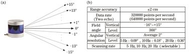
Fig. 1. Basic parameters and basic principles of LiDAR. (a) Schematic diagram of laser emission; (b)basic parameters

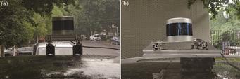
Fig. 2. LiDAR installation schematic. (a) Front view; (b) side view

Fig. 3. Vehicle and LiDAR coordinate systems

Fig. 4. Cloud diagram of the vehicle turning to the right to the tunnel point

Fig. 5. Point cloud in the longitudinal reference direction of the tunnel. (a) Two-dimensional schematic diagram of point cloud; (b) three-dimensional schematic diagram of point cloud; (c) LiDAR point cloud with vertical field angle of 1°; (d) point cloud in the longitudinal reference direction of the tunnel

Fig. 6. Particle group algorithm flow diagram

Fig. 7. Top view of point cloud coordinate conversion of tunnel wall. (a) Original point cloud; (b) post-conversion point cloud; (c) comparison chart

Fig. 8. Tunnel cross-section point cloud

Fig. 9. Fitting effect diagrams. (a) Particle swarm optimization algorithm; (b) least squares method (circle); (c) least squares method (ellipse)

Fig. 10. LiDAR installation diagram. (a) Front view; (b) side view

Fig. 11. Point cloud of cross section of tunnel

Fig. 12. Test results. (a) Original point cloud; (b) converted point cloud; (c) center point of tunnel cross section; (d) fitting result of tunnel centerline

Table 1.

Table 2.