Memory-assisted quantum accelerometer with multi-bandwidth

Zhifei Yu; Bo Fang; Liqing Chen; Keye Zhang; Chun-Hua Yuan; Weiping Zhang

doi:10.1364/PRJ.453940

Abstract

The accelerometer plays a crucial role in inertial navigation. The performance of conventional accelerometers such as lasers is usually limited by the sensing elements and shot noise limitation (SNL). Here, we propose an advanced development of an accelerometer based on atom–light quantum correlation, which is composed of a cold atomic ensemble, light beams, and an atomic vapor cell. The cold atomic ensemble, prepared in a magneto-optical trap and free-falling in a vacuum chamber, interacts with light beams to generate atom–light quantum correlation. The atomic vapor cell is used as both a memory element storing the correlated photons emitted from cold atoms and a bandwidth controller through the control of free evolution time. Instead of using a conventional sensing element, the proposed accelerometer employs interference between quantum-correlated atoms and light to measure acceleration. Sensitivity below SNL can be achieved due to atom–light quantum correlation, even in the presence of optical loss and atomic decoherence. Sensitivity can be achieved at the

ng / \sqrt{Hz}

level, based on evaluation via practical experimental conditions. The present design has a number of significant advantages over conventional accelerometers such as SNL-broken sensitivity, broad bandwidth from a few hundred Hz to near MHz, and avoidance of the technical restrictions of conventional sensing elements.

1. INTRODUCTION

Accelerometers have extensively been applied as weak force probes, especially in situations that involve inertial navigation, land-based resource exploration, and seismic monitoring [1 –4]. There are many types of accelerometers, including capacitive [5,6], piezoelectric [7], tunnel-current [8], thermal [9], and optical [10 –16]. Almost all utilize mass-spring-damper systems as displacement sensors [17]. The performance of such accelerometers highly relies on fabrication of the displacement sensors, which directly results in technical limitations to the bandwidth, quality factor $Q_{f}$ , and noise level [18]. Among numerous accelerometers, optical ones have attracted much attention due to their high sensitivity. However, the sensitivity of such accelerometers is fundamentally subject to shot noise limitation (SNL) [19,20]. Developing methods and technologies to break the SNL and remove the technical limitations of conventional displacement sensors is desired for the innovation of accelerometers.

In this paper, we present a memory-assisted quantum accelerometer (MQA), which consists of atomic ensembles, light beams, and optical elements. The MQA has three advantages over conventional accelerometers. First, instead of a mass-spring-damper system, a cold atomic ensemble [21] acts as the displacement sensor, which can avoid the technical restrictions of a mass-spring-damper system. Second, the SNL-broken sensitivity in measurement of acceleration can be achieved by the quantum interference of correlated atoms and light [22 –24]. The third merit is that the accelerometer allows a tunable bandwidth, which is determined by the controllable memory time $t_{M}$ of the correlated photons stored in a memory element [25 –27]. We calculate and analyze the sensitivity and bandwidth of the MQA. An inverse relation exists between sensitivity and bandwidth. Sensitivity can reach below the SNL in the range of bandwidth from a few hundred Hz to near MHz due to atom–light quantum correlation, even in the presence of the optical losses and atomic decoherence. An optimal $ng / \sqrt{Hz}$ -level sensitivity without loss is anticipated at frequencies $\sim 100 Hz$ for a feasible average atomic number and an available memory time $t_{M} = 10 ms$ .

2. RESULTS

A. Principle of MQA

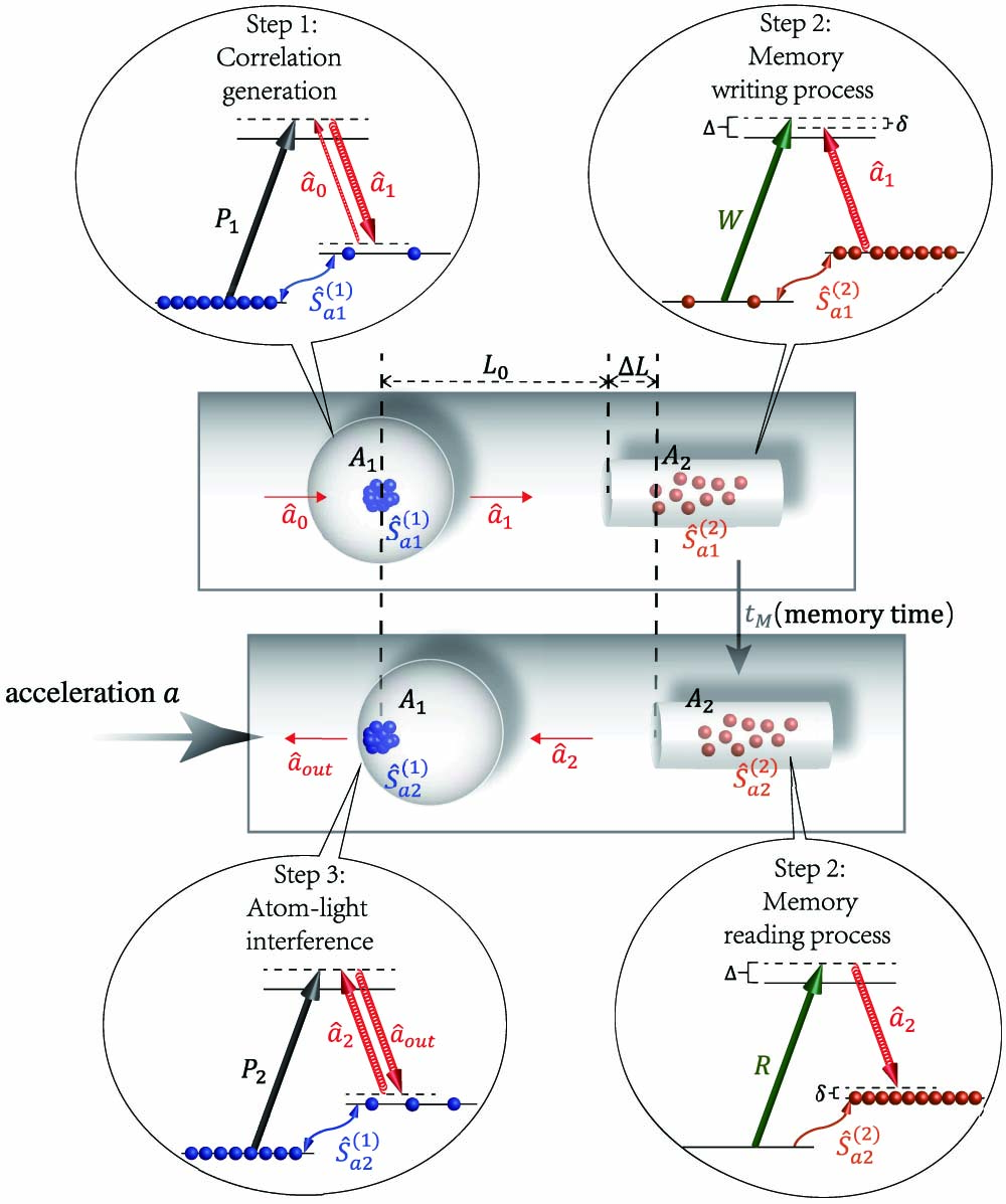
A schematic diagram of the accelerometer is shown in Fig. 1. The cores are composed of two atomic systems: cold ensemble $A_{1}$ and atomic vapor cell $A_{2}$ . $A_{1}$ is prepared in a magneto-optical trap (MOT), free-falling in the vacuum chamber to generate atom ( ${\hat{S}}_{a_{1}}^{(1)}$ )–light ( ${\hat{a}}_{1}$ ) quantum correlation and realize atom–light interference via two Raman scattering processes. Atomic vapor cell $A_{2}$ , containing thermal atoms and buffer gas, is a memory element to store the correlated photonic signal ${\hat{a}}_{1}$ from $A_{1}$ , which acts as a bandwidth modulator. In principle, the memory element can be any quantum memorizer for photons with long coherence times, such as rare-earth-doped crystals [28,29]. All optical devices including the vacuum chamber and memory element are fixed onto a mobile platform. When MOT is turned on, $A_{1}$ and $A_{2}$ move together with the platform. The distance $L$ between two atomic systems is fixed as $L_{0}$ at any velocity or acceleration of the platform. When MOT is turned off, $A_{1}$ is free-falling in vacuum, acting as the static frame reference, and $A_{2}$ remains moving with the platform at acceleration $a$ . $L = L_{0} + Δ L$ changes with acceleration, where $Δ L$ is the displacement due to acceleration $a$ . $Δ L = \frac{1}{2} a T^{2}$ , where $T$ is the free-evolution time duration after the first Raman scattering process and before the second one, that is, the atom–light “wave-splitting” and “wave-recombining” processes, respectively. $T$ is independent of acceleration $a$ and the velocity of the platform. $Δ L$ can be achieved via atom–light quantum interference. Acceleration $a$ can be achieved by the variation of $Δ L$ with time $T$ . The acceleration sensitivity is no longer limited by the performance of the mass-spring-damper system. This is one of the advantages of our scheme.

Sign up for Photonics Research TOC. Get the latest issue of Photonics Research delivered right to you！Sign up now

Figure 1.Schematic diagram of the MQA. The cold atomic ensemble $A_{1}$ is free-falling in the vacuum chamber. Atomic vapor $A_{2}$ , the vacuum chamber, and all optical elements are fixed on and move with the platform at acceleration $a$ . The distance between $A_{1}$ and $A_{2}$ is changed from $L_{0}$ to $L_{0} + Δ L$ . $Δ L$ is the acceleration-dependent displacement achieved via atom–light quantum interference, which is realized in three steps. Step 1: ${\hat{a}}_{1}$ and ${\hat{S}}_{a_{1}}^{(1)}$ are generated by the first stimulated Raman scattering (SRS) in $A_{1}$ via input seed ${\hat{a}}_{0}$ and Raman pump $P_{1}$ . The atomic spin wave is ${\hat{S}}_{a_{j}}^{(i)}$ , where superscript $i$ ( $i = 1$ , 2) indicates different atomic ensemble $A_{1}$ or $A_{2}$ , and subscript $j$ ( $j = 1$ , 2, 3) represents the evolution state at different times of atomic ensemble $A_{i}$ . Step 2: ${\hat{a}}_{1}$ is stored in $A_{2}$ as ${\hat{S}}_{a_{1}}^{(2)}$ is driven by the strong write pulse $W$ . After memory time $t_{M}$ , ${\hat{S}}_{a_{2}}^{(2)}$ , evolved from ${\hat{S}}_{a_{1}}^{(2)}$ due to atomic decay, is retrieved back to ${\hat{a}}_{2}$ by the read pulse $R$ . Step 3: ${\hat{S}}_{a_{2}}^{(1)}$ , evolved from ${\hat{S}}_{a_{1}}^{(1)}$ during the memory time, and ${\hat{a}}_{2}$ interfere by the second SRS via Raman pump $P_{2}$ .

The accelerometer is operated in three steps: generation of atom–light quantum correlation via the first Raman scattering in $A_{1}$ , atomic memory in $A_{2}$ , and acceleration acquisition via atom–light interference. Below, we describe the calculation and analysis in detail.

B. Generation of Quantum Correlation

Atom–light quantum correlation is generated via stimulated Raman scattering (SRS) in $A_{1}$ , which is effectively an atom–light wave-splitting process. A Stokes seed ${\hat{a}}_{0}$ and a strong Raman beam $P_{1}$ interact with the atoms in $A_{1}$ to generate Stokes light ${\hat{a}}_{1}$ and atomic spin wave ${\hat{S}}_{a_{1}}^{(1)}$ [30]. The input–output relation of SRS can be written as ${\hat{a}}_{1} = G_{1} {\hat{a}}_{0} + g_{1} {\hat{S}}_{a_{0}}^{(1) †} e^{i θ_{P_{1}}}$ , ${\hat{S}}_{a_{1}}^{(1)} = G_{1} {\hat{S}}_{a_{0}}^{(1)} + g_{1} {\hat{a}}_{0}^{†} e^{i θ_{P_{1}}}$ . ${\hat{S}}_{a_{0}}^{(1)}$ describes the initial spin wave, which starts from the ground state of the atomic ensemble. $G_{1}$ and $g_{1}$ are Raman gains that satisfy $G_{1}^{2} = g_{1}^{2} + 1$ , and $θ_{P_{1}}$ is the phase of beam $P_{1}$ .

After SRS, the generated Stokes signal ${\hat{a}}_{1}$ , transmitting out of $A_{1}$ and entering $A_{2}$ , quantum-mechanically correlates with the induced atomic spin wave ${\hat{S}}_{a_{1}}^{(1)}$ that remains in $A_{1}$ . The intensity fluctuations of both ${\hat{a}}_{1}$ and ${\hat{S}}_{a_{1}}^{(1)}$ are amplified to the level above SNL as a result of Raman amplification. But the relative intensity fluctuation ${\hat{S}}_{a_{1}}^{(1) †} {\hat{S}}_{a_{1}}^{(1)} - {\hat{a}}_{1}^{†} {\hat{a}}_{1}$ is squeezed below SNL by $2 G_{1}^{2} - 1$ times, due to the quantum correlation between ${\hat{a}}_{1}$ and ${\hat{S}}_{a_{1}}^{(1)}$ (see Appendix A).

C. Atomic Memory

Stokes signal ${\hat{a}}_{1}$ propagates into atomic vapor cell $A_{2}$ , and then is stored as atomic spin wave ${\hat{S}}_{a_{1}}^{(2)}$ in the writing process driven by the write beam $W$ . The evolution of the spin wave obeys the Heisenberg propagation equation $\frac{\partial}{\partial t} {\hat{S}}_{a_{1}}^{(2)} = - i (\frac{{| Ω_{W} |}^{2}}{Δ} - δ + Δ k_{W} \cdot v) {\hat{S}}_{a_{1}}^{(2)} - i χ {\hat{a}}_{1},$ (1)where $Ω_{W}$ is the Rabi frequency of $W$ , $Δ$ is single-photon detuning, $δ$ is two-photon detuning, $Δ k_{W} = k_{W} - k_{s}$ is the wave vector difference of $W$ and ${\hat{a}}_{1}$ , $χ$ is the Raman coupling coefficient, $v$ is the center of mass velocity of the atoms, and $Δ k_{W} \cdot v$ is the Doppler frequency shift. The solution to Eq. (1) is (see Appendix B) ${\hat{S}}_{a_{1}}^{(2)} = (- i \sqrt{η_{W}} e^{i θ_{W}} {\hat{a}}_{1} e^{i φ} + e^{i θ_{W_{0}}} \sqrt{1 - η_{W}} {\hat{S}}_{a_{0}}^{(2)}) \times e^{- i (\frac{{| Ω_{W} |}^{2}}{Δ} - δ + Δ k_{W} \cdot v) t_{W} / 2},$ (2)where $η_{W}$ is the writing efficiency determined by the coupling coefficient $χ$ ; $φ = k_{s} L_{0}$ , and $k_{s} = 2 π / λ_{s}$ , with $λ_{s}$ the Stokes wavelength. $θ_{W}$ is the phase of the write field $W$ ; $t_{W}$ is the writing time. ${\hat{S}}_{a_{0}}^{(2)}$ is the initial spin wave in $A_{2}$ , which is in the vacuum state. The term $\frac{{| Ω_{W} |}^{2}}{Δ}$ corresponds to the Stark effect. $\frac{{| Ω_{W} |}^{2}}{Δ}$ , $δ$ , and $θ_{W_{0}}$ are acceleration-independent parameters, which can be considered as fixed values.

After memory time $t_{M}$ , ${\hat{S}}_{a_{2}}^{(2)}$ , evolving from ${\hat{S}}_{a_{1}}^{(2)}$ with decay rate $Γ_{2}$ due to atomic collisions, can be read out as Stokes ${\hat{a}}_{2}$ with efficiency $η_{R}$ by the read beam $R$ . Assuming a reading time $t_{R} \sim t_{W}$ and defining $η = η_{W} η_{R}$ , Stokes ${\hat{a}}_{2}$ can be simplified as (see Appendix C) ${\hat{a}}_{2} = - \sqrt{η} e^{- i (Δ φ_{a} + Δ φ_{v} - φ_{0})} e^{- Γ_{2} t_{M}} {\hat{a}}_{1} + \sqrt{1 - η e^{- 2 Γ_{2} t_{M}}} \hat{V},$ (3)where $\hat{V}$ is the effective vacuum field. The phase offset $φ_{0}$ can be safely set to zero since it is independent of the measured acceleration $a$ (see Appendix C). The velocity-dependent phase shift $Δ φ_{v} = Δ k_{W} \cdot v t_{M}$ is induced by the Doppler effect due to the center of mass motion of atoms. The acceleration-dependent phase shift $Δ φ_{a} \equiv Δ k a t_{M} (t_{M} - t_{W}) / 2 - k_{s} (Δ L)$ , where $Δ k$ is the projection of $Δ k_{W}$ along the acceleration. $Δ L = \frac{1}{2} a T^{2} = \frac{1}{2} a {(t_{1} + t_{2} + t_{M})}^{2}$ , where $t_{1}$ and $t_{2}$ are the flying times of the Stokes light between cold ensemble $A_{1}$ and vapor cell $A_{2}$ forth and back, respectively. Normally, $k_{s} ≫ | Δ k |$ and $t_{M} ≫ t_{W, R} ≫ t_{1,2}$ , i.e., $Δ φ_{a} ≃ - k_{s} a t_{M}^{2} / 2$ . The phase shift of the Stokes field can be measured through atom–light interference between the readout field ${\hat{a}}_{2}$ returning to $A_{1}$ and atomic spin wave ${\hat{S}}_{a_{1}}^{(1)}$ remaining in $A_{1}$ .

D. Atom–Light Interference

When $a_{2}$ returns to $A_{1}$ , the atomic spin wave ${\hat{S}}_{a_{1}}^{(1)}$ has experienced free evolution for the duration of memory time $t_{M}$ . As a result, the spin wave has the form ${\hat{S}}_{a_{2}}^{(1)} = {\hat{S}}_{a_{1}}^{(1)} e^{- Γ_{1} t_{M}} + {\hat{F}}^{(1)}$ , with Doppler dephasing being negligible in the cold ensemble (see Appendix D), where ${\hat{F}}^{(1)}$ is the quantum Langevin operator, reflecting the collision-induced fluctuation and satisfying $[{\hat{F}}^{(1)}, {\hat{F}}^{(1) †}] = 1 - e^{- 2 Γ_{1} t_{M}}$ [24]. The decay rate $Γ_{1}$ represents the decoherence effect due to atomic collisions and flying off the laser beam. For a general cold atomic ensemble, the root mean square velocity is ∼ several cm/s, and the diffusion of cold atoms is $\sim 1.0 mm$ after a memory time of 10 ms. The whole atomic ensemble will drop 0.5 mm in gravity direction after 10 ms. The mismatch of the spot expansion and dropping of the cold atomic ensemble plays an opposite role in quantum enhancement by destroying atom–light quantum correlation. However, these two effects can be solved using laser beam expansion and light path adjustment in the experiment.

${\hat{a}}_{2}$ and ${\hat{S}}_{a_{2}}^{(1)}$ interact with each other in $A_{1}$ , which is driven by $P_{2}$ with $θ_{P_{2}} = θ_{P_{1}}$ , and generate Stokes ${\hat{a}}_{out}$ with atomic spin wave ${\hat{S}}_{a_{out}}^{(1)}$ by a second Raman scattering. Setting $\sqrt{T_{1}} \equiv e^{- Γ_{1} t_{M}}$ and $\sqrt{T_{2}} \equiv e^{- Γ_{2} t_{M}}$ , we have the final output ${\hat{a}}_{out} = ς_{1} {\hat{a}}_{0} + ς_{2} {\hat{S}}_{a_{0}}^{(1) †} + ς_{3} \hat{V} + ς_{4} {\hat{f}}^{†}$ (see Appendix D), where $\hat{f}$ is the normalized noise operator, $\hat{f} \equiv {\hat{F}}^{(1)} / \sqrt{1 - T_{1}}$ , $ς_{1} \equiv g_{1} g_{2} \sqrt{T_{1}} - G_{1} G_{2} \sqrt{η T_{2}} e^{i (Δ φ_{a} + Δ φ_{v})}$ , $ς_{2} \equiv e^{i θ_{P_{2}}} [G_{1} g_{2} \sqrt{T_{1}} - g_{1} G_{2} \sqrt{η T_{2}} e^{i (Δ φ_{a} + Δ φ_{v})}]$ , $ς_{3} \equiv G_{2} \sqrt{1 - η T_{2}}$ , and $ς_{4} \equiv g_{2} e^{i θ_{P_{2}}} \sqrt{1 - T_{1}}$ .

Here, we emphasize that atomic vapor cell $A_{2}$ moves with the platform. To achieve acceleration, this requires that the vapor atoms and cell wall move as a whole, which implies that a robust thermal equilibrium between the atoms and the cell wall is essential during memory time. This is realized with the assistance of buffer gas in the vapor cell. In a room-temperature cell with buffer gas at several-Torr pressure, the mean free path of atoms is $\sim μm$ , with $v_{rms} \sim 300 m/s$ . This allows the vapor atoms to remain in thermal equilibrium with the cell wall under acceleration (see Appendix D). The ground-state coherence can be preserved for up to $10^{8}$ collisions between the buffer gas and atoms [31]. The buffer gas can separate atoms and decrease the collision between them. Therefore, the value of the decay rate $Γ_{2}$ is small [32]. Doppler dephasing ( $Δ φ_{v}$ ) can be avoided by adopting near-degenerate Zeeman two-photon transitions, as shown in Appendix E. Now the Stokes field ${\hat{a}}_{out}$ , containing only phase $Δ φ_{a}$ , can be measured through homodyne detection (HD).

E. Acquisition of Acceleration

All optical devices including the vacuum chamber and memory element are fixed onto a mobile platform. When MOT is turned on, cold ensemble $A_{1}$ and atomic vapor cell $A_{2}$ move together with the platform. The distance $L$ between two atomic systems is fixed as $L_{0}$ at any velocity $v_{0}$ or acceleration of platform $a$ . When MOT is turned off, the movement of the cold atomic ensemble is independent of the platform. The cold atomic ensemble moves in uniform motion with constant velocity $v_{0}$ . The atomic vapor still moves with the platform under acceleration. Its velocity changes with acceleration, and the distance between two atomic systems also changes from $L_{0}$ to $L_{0} + Δ L$ , where $Δ L = Δ v_{0} T + \frac{1}{2} a T^{2}$ is the displacement due to acceleration, with $Δ v_{0}$ the initial relative velocity of $A_{1}$ and $A_{2}$ , and $T$ is independent of the acceleration $a$ and velocity of the platform. $Δ L$ causes a phase shift. Here, $Δ v_{0}$ is zero because the velocities of two atomic systems are the same before MOT is turned off. Acceleration can be measured in the direction of the seed and pump fields passing the cold ensemble, and it can be expressed in terms of the phase $Δ φ_{a}$ as follows: $a = \frac{λ_{s} Δ φ_{a}}{π t_{M}^{2}} .$ (4)

Using the HD of the quadrature of Stokes field ${\hat{a}}_{out}$ , acceleration is measured, and sensitivity is given by (see Appendix E) $Δ a = \frac{1}{Q_{e}} Δ a_{SNL},$ (5)where $Q_{e}$ is the quantum enhancement factor. Sensitivity breaks the SNL when $Q_{e} > 1$ . In general, $Q_{e} = \frac{2 G_{1} G_{2}}{\sqrt{G_{1}^{2} + g_{1}^{2}}} \frac{\sqrt{η} e^{- Γ_{2} t_{M}}}{\sqrt{\sum_{n = 1}^{4} {| ς_{n}^{0} |}^{2}}},$ (6)where $ς_{n}^{0}$ are the values of $ς_{n} (n = 1, \dots,4)$ at the dark fringe. Defining $N_{0} \equiv ⟨ {\hat{a}}_{0}^{†} {\hat{a}}_{0} ⟩$ for the input mean photon number, we work out the SNL for acceleration measurement: $Δ a_{SNL} = \frac{λ_{s}}{π \sqrt{(G_{1}^{2} N_{0} + g_{1}^{2} N_{0})} t_{M}^{2}},$ (7)where $G_{1}^{2} N_{0}$ and $g_{1}^{2} N_{0}$ are the particle numbers of Stokes signal ${\hat{a}}_{1}$ and atomic spin wave ${\hat{S}}_{a_{1}}^{(1)}$ , respectively. Acceleration sensitivity depends on the phase sensitivity of atom–light interference, whose SNL is determined by the total phase-sensitive particle number $(G_{1}^{2} + g_{1}^{2}) N_{0}$ of two interference beams, signal ${\hat{a}}_{1}$ and atomic spin wave ${\hat{S}}_{a_{1}}^{(1)}$ . Here, quantum correlation between ${\hat{S}}_{a_{1}}^{(1)}$ and ${\hat{a}}_{1}$ is key to breaking the SNL in acceleration sensitivity.

F. Accelerometer Sensitivity

To obtain the best sensitivity in the acceleration measurement, it is essential to decrease $Δ a_{SNL}$ itself and increase quantum enhancement factor $Q_{e}$ . In general, $Δ a_{SNL}$ can be reduced by increasing the input particle number $N_{0}$ and prolonging memory time $t_{M}$ . However, this is usually constrained in realistic experiments. In this sense, quantum enhancement provides just an alternative way to further improve sensitivity through SNL breaking.

Factor $Q_{e}$ is complicated, and we numerically analyze the behavior of $Q_{e}$ in Fig. 2(a) as a function of $T_{1}$ and $T_{2}^{'}$ ( $T_{2}^{'} \equiv η T_{2}$ ) for a different Raman gain $G_{2}$ under a given $G_{1}$ . The larger $T_{1}$ , $T_{2}^{'}$ , and $G_{2}$ , the larger $Q_{e}$ . The red solid curves with $Q_{e} = 1$ in Fig. 2(a) set a critical boundary of the SNL, which reflects a balance of competition between losses and quantum correlation. The region within the curves marks $Q_{e} > 1$ , representing quantum enhancement.

Figure 2.(a) Quantum enhancement factor $Q_{e}$ versus $T_{1}$ and $T_{2}^{'}$ when $G_{2} = 2$ and 8, respectively. (b) Sensitivity versus $s$ and $G_{2}$ when $T_{1} = 0.5$ and $1$ , respectively. $s = T_{2}^{'} / T_{1}$ is the ratio of two beams’ losses. The red curves mark $Q_{e} = 1$ for SNL. Sensitivities within the red curves can beat the SNL. Parameter settings: $N_{0} {= 10}^{6}$ , $G_{1} = 8$ , $λ_{s} = 795 nm$ , and $t_{M} = 1 ms$ .

On the other hand, in terms of Eq. (7), the gains $G_{1}$ , $g_{1}$ , and $N_{0}$ determine the SNL for acceleration sensitivity. To set an SNL as low as possible in the measurement, it is essential to achieve gains as high as possible. Hence, we assume $G_{1} ≫ 1$ for numeric analysis. Sensitivity $Δ a$ is shown as a function of $s = T_{2}^{'} / T_{1}$ and $G_{2}$ under given $G_{1}$ and $N_{0}$ in Fig. 2(b). The quantum enhancing region associated with $Q_{e} > 1$ is marked as the same within the red solid curves. Obviously, high gain $G_{2}$ and low losses can greatly enhance sensitivity due to the sufficient exploitation of quantum correlation. In addition, quantum enhancement of sensitivity well exhibits a loss tolerance, and highly depends on the balance of losses defined by the ratio $s$ . The best sensitivity appears near $s = 1$ for high gains, where the atomic and optical losses are well balanced. In particular, sensitivity can keep beating the SNL through quantum enhancement until losses approach the limit $T_{1} \sim T_{2}^{'} \sim 0.5$ .

G. Measurement Bandwidth

Sensitivity $Δ a$ is the result determined by one single-shot measurement approximately completed in memory time $t_{M}$ , which gives the upper limit of the MQA’s frequency $f_{\max} = 1 / t_{M}$ . In realistic experiments, if the setup of the system takes time $t_{s}$ , and stable operation for $M$ -times repeating measurements takes time $t_{o} = M t_{M}$ , then the overall sensitivity of the accelerometer is given by $Δ a_{o} \equiv Δ a / \sqrt{f_{eff}} \propto {(f_{\max})}^{3 / 2}$ , where $f_{eff} = f_{\max} t_{o} / (t_{s} + t_{o})$ .

There is a trade-off between sensitivity $Δ a_{o}$ and bandwidth, as shown in Fig. 3. In general, sensitivity $Δ a_{o}$ has a 3/2 power-law dependence of bandwidth, indicating that sensitivity degrades in the high-frequency region. In Fig. 3, we see that when the losses of the system remain low enough, the accelerometer exhibits well the quantum advantage to achieve an SNL below sensitivity with a broad range of frequencies. Sensitivity rises above the SNL at low frequencies with losses. As a comparison, some available data of sensitivities for previously reported accelerometers are labeled in Fig. 3 as well. Overall, the MQA has great potential in highly-sensitive measurements of acceleration.

Figure 3.Sensitivity as a function of bandwidth under the conditions $G = 8$ , $N_{0} {= 10}^{6}$ , $λ_{s} = 795 nm$ , and $η = 1$ . The data of other reported accelerometers are given as comparison. Dark green diamond: microchip optomechanical accelerometer [14]. Orange pentagram: micromechanical capacitive accelerometer [18]. Purple hexagram: MEMS accelerometer [6]. Gray circle: optical accelerometer [15].

With the available experimental conditions, e.g., $N_{0} {= 10}^{6}$ per pulse, Raman gain $G_{1} = 8$ , $G_{2} = 2$ , MOT cycle $t_{s} = 30 ms$ [33,34], memory time $t_{M} \sim 10 ms$ [35,36], we can achieve single-shot sensitivity 23 ng at frequency 100 Hz. Finally, the sensitivity is $\sim 4.6 ng / \sqrt{Hz}$ .

For the traditional interferometric accelerometer, the only method to improve sensitivity at a high bandwidth is to increase the quality factor $Q_{f}$ of the damper, which is technically hard to implement. In our scheme, sensitivity at a high bandwidth can be improved by increasing the Raman gain or the number of initial photons and trapping cold atoms, making it much easier to operate.

3. DISCUSSION AND CONCLUSION

We present an innovative principle for a quantum enhanced accelerometer. There are several significant advantages over other interferometer-based accelerometers: broad bandwidth, SNL below sensitivity, and mechanics-free sensing flexibility compared to mass-spring-damper systems. The dynamic range of acceleration depends on that of phase measurement, which is from the phase sensitivity to $2 π$ . With $λ_{s}$ of 795 nm, the dynamic range of acceleration of a single shot is from 23 ng to 1.59 mg with $t_{M} = 10 ms$ , and from $2.3 g$ to $1.59 \times 10^{5} g$ with $t_{M} = 1.0 μs$ . It can be seen that the dynamic range is $\sim 48 dB$ with a fixed $t_{M}$ . Furthermore, the measurable range of acceleration is from 23 ng to $1.59 \times 10^{5} g$ , $\sim 128 dB$ , only by adjusting $t_{M}$ to suitable values. In future applications of the MQA, a long atomic coherence time of $A_{1,2}$ and high memory efficiency $η$ are crucial to achieve high sensitivity. Large optical depths for $A_{1,2}$ are required to ensure enough atomic numbers to achieve a large input particle number $N_{0}$ and high gains, so as to lower the level of $Δ a_{SNL}$ and raise the quantum enhancement factor $Q_{e}$ .

We emphasize that this work building the MQA is based on quantum correlation. The physics behind this is universal. Hence, the principle presented in this paper is not limited only to the atom–light coupling system, but can be extended to other systems that can generate and preserve quantum correlation, such as rare-earth-doped crystals [28,29]. Specifically, one crystal can be trapped and released to generate light–crystal correlation. The other crystal, fixed on platform, acts as the quantum memorizer. Acceleration sensitivity also depends on the phase-sensitive particle number and memory time.

APPENDIX A: GENERATION OF QUANTUM CORRELATION

P_{1}

A_{1}

DOS = \frac{⟨ {\hat{a}}_{0}^{†} {\hat{a}}_{0} ⟩}{(2 G_{1}^{2} - 1) ⟨ {\hat{a}}_{0}^{†} {\hat{a}}_{0} ⟩} = \frac{1}{2 G_{1}^{2} - 1} .

{\hat{a}}_{1}

APPENDIX B: MEMORY PROCESS

H = ℏ χ \hat{a} {\hat{S}}_{a}^{†} + h .c .,

APPENDIX C: READOUT PROCESS

Ω_{R}

{\hat{a}}_{2}

Ω_{W} = Ω_{R}

APPENDIX D: ATOM–LIGHT INTERFERENCE

{\hat{S}}_{a_{1}}^{(1)}

{\hat{a}}_{2}

APPENDIX E: ACCELERATION SENSITIVITY USING HOMODYNE DETECTION

A_{1}

Δ a = \frac{λ_{s}}{π t_{M}^{2}} \frac{{⟨ {(Δ \hat{O})}^{2} ⟩}^{1 / 2}}{| \partial \hat{O} / \partial φ |},

{\hat{a}}_{out}

{\hat{a}}_{0}

⟨ Δ^{2} \hat{X} ⟩ = {| ς_{1} |}^{2} + {| ς_{2} |}^{2} + {| ς_{3} |}^{2} + {| ς_{4} |}^{2},

e^{- Γ_{1} t_{M}}

Δ a = \frac{λ_{s}}{π t_{M}^{2}} \frac{\sqrt{⟨ Δ^{2} \hat{X} ⟩}}{| \frac{\partial ⟨ \hat{X} ⟩}{\partial (Δ φ_{a})} |} = \frac{1}{Q_{e}} Δ a_{SNL},

References

[1] P. S. de Brito Andre, H. Varum. Accelerometers: Principles, Structure and Applications(2013).

[2] M. Bao. Micro Mechanical Transducers: Pressure Sensors, Accelerometers and Gyroscopes(2000).

[3] C.-W. Tan, S. Park. Design of accelerometer-based inertial navigation systems. IEEE Trans. Instrum. Meas., 54, 2520-2530(2005).

[4] D. Jiang, W. Zhang, F. Li. All-metal optical fiber accelerometer with low transverse sensitivity for seismic monitoring. IEEE Sens. J., 13, 4556-4560(2013).

[5] C. Acar, A. M. Shkel. Experimental evaluation and comparative analysis of commercial variable-capacitance MEMS accelerometers. J. Micromech. Microeng., 13, 634-645(2003).

[6] Y. Dong, P. Zwahlen, A. M. Nguyen, R. Frosio, F. Rudolf. Ultra-high precision MEMS accelerometer. 16th International Solid-State Sensors, Actuators and Microsystems Conference, 695-698(2011).

[7] S. Tadigadapa, K. Mateti. Piezoelectric MEMS sensors: state-of-the-art and perspectives. Meas. Sci. Technol., 20, 092001(2009).

[8] C. Liu, A. M. Barzilai, J. K. Reynolds, A. Partridge, T. W. Kenny, J. D. Grade, H. K. Rockstad. Characterization of a high-sensitivity micromachined tunneling accelerometer with micro-g resolution. J. Microelectromech. Syst., 7, 235-244(1998).

[9] R. Mukherjee, J. Basu, P. Mandal, P. K. Guha. A review of micromachined thermal accelerometers. J. Micromech. Microeng., 27, 123002(2017).

[10] U. Krishnamoorthy, R. H. Olsson, G. R. Bogart, M. S. Baker, D. W. Carr, T. P. Swiler, P. J. Clews. Inplane MEMS-based nano-g accelerometer with sub-wavelength optical resonant sensor. Sens. Actuators A Phys., 145, 283-290(2008).

[11] K. Zandi, B. Wong, J. Zou, R. V. Kruzelecky, W. Jamroz, Y. Peter. In-plane silicon-on-insulator optical MEMS accelerometer using waveguide Fabry-Perot microcavity with silicon/air Bragg mirror. IEEE 23rd International Conference on Micro Electro Mechanical Systems (MEMS), 839-842(2010).

[12] W. Noell. Applications of SOI-based optical MEMS. IEEE J. Sel. Top. Quantum Electron., 8, 148-154(2002).

[13] T. A. Berkoff, A. D. Kersey. Experimental demonstration of a fiber Bragg grating accelerometer. IEEE Photon. Technol. Lett., 8, 1677-1679(1996).

[14] A. G. Krause, M. Winger, T. D. Blasius, Q. Lin, O. Painter. A microchip optomechanical accelerometer. Nat. Photonics, 6, 768-772(2012).

[15] Y. Yang, X. Li, K. Kou, L. Zhang. Optical accelerometer design based on laser self-mixing interference. Proc. SPIE, 9369, 93690R(2015).

[16] Y. L. Li, P. F. Barker. Characterization and testing of a micro-g whispering gallery mode optomechanical accelerometer. J. Lightwave Technol., 36, 3919-3926(2018).

[17] N. Lagakos, T. Litovitz, P. Macedo, R. Mohr, R. Meister. Multimode optical fiber displacement sensor. Appl. Opt., 20, 167-168(1981).

[18] S. Chen, H. Xu. Design analysis of a high-Q micromechanical capacitive accelerometer system. IEICE Electron. Express, 14, 20170410(2017).

[19] M. D. LeHaye, O. Buu, B. Camarota, K. C. Schwab. Approaching the quantum limit of a nanomechanical resonator. Science, 304, 74-77(2004).

[20] J. P. Dowling. Quantum optical metrology-the lowdown on high-N00N states. Contemp. Phys., 49, 125-143(2008).

[21] P. Qian, Z. Gu, R. Cao, R. Wen, Z. Y. Ou, J. F. Chen, W. Zhang. Temporal purity and quantum interference of single photons from two independent cold atomic ensembles. Phys. Rev. Lett., 117, 013602(2016).

[22] B. Chen, C. Qiu, S. Chen, J. Guo, L. Q. Chen, Z. Y. Ou, W. Zhang. Atom-light hybrid interferometer. Phys. Rev. Lett., 115, 043602(2015).

[23] X. Feng, Z. Yu, B. Chen, S. Chen, Y. Wu, D. Fan, C.-H. Yuan, L. Q. Chen, Z. Y. Ou, W. Zhang. Reducing the mode-mismatch noises in atom-light interactions via optimization of the temporal waveform. Photon. Res., 8, 1697-1702(2020).

[24] Z.-D. Chen, C.-H. Yuan, H.-M. Ma, D. Li, L. Q. Chen, Z. Y. Ou, W. Zhang. Effects of losses in the atom-light hybrid SU(1,1) interferometer. Opt. Express, 24, 17766-17778(2016).

[25] C. Liu, Z. Dutton, C. H. Behroozi, L. V. Hau. Observation of coherent optical information storage in an atomic medium using halted light pulses. Nature, 409, 490-493(2001).

[26] M. Hosseini, B. M. Sparkes, G. Campbell, P. K. Lam, B. C. Buchler. High efficiency coherent optical memory with warm rubidium vapour. Nat. Commun., 2, 174(2011).

[27] J. Guo, X. Feng, P. Yang, Z. Yu, L. Q. Chen, C.-H. Yuan, W. Zhang. High-performance Raman quantum memory with optimal control in room temperature atoms. Nat. Commun., 10, 148(2019).

[28] Y. Ma, Y.-Z. Ma, Z.-Q. Zhou, C.-F. Li, G.-C. Guo. One-hour coherent optical storage in an atomic frequency comb memory. Nat. Commun., 12, 2381(2021).

[29] M. Zhong, M. P. Hedges, R. L. Ahlefeldt, J. G. Bartholomew, S. E. Beavan, S. M. Wittig, J. J. Longdell, M. J. Sellars. Optically addressable nuclear spins in a solid with a six-hour coherence time. Nature, 517, 177-180(2015).

[30] C. H. van der Wal, M. D. Eisaman, A. André, R. L. Walsworth, D. F. Phillips, A. S. Zibrov, M. D. Lukin. Atomic memory for correlated photon states. Science, 301, 196-200(2003).

[31] W. Happer. Optical pumping. Rev. Mod. Phys., 44, 169-249(1972).

[32] S. Manz, T. Fernholz, J. Schmiedmayer, J.-W. Pan. Collisional decoherence during writing and reading quantum states. Phys. Rev. A, 75, 040101(2007).

[33] S. Zhang, J. F. Chen, C. Liu, S. Zhou, M. M. T. Loy, G. K. L. Wong, S. Du. A dark-line two-dimensional magneto optical trap of ⁸⁵Rb atoms with high optical depth. Rev. Sci. Instrum., 83, 073102(2012).

[34] A. G. Radnaev, Y. O. Dudin, R. Zhao, H. H. Jen, S. D. Jenkins, A. Kuzmich, T. A. B. Kennedy. A quantum memory with telecom-wavelength conversion. Nat. Phys., 6, 894-899(2010).

[35] X.-H. Bao, A. Reingruber, P. Dietrich, J. Rui, A. Duck, T. Strasse, L. Li, N.-L. Liu, B. Zhao, J.-W. Pan. Efficient and long-lived quantum memory with cold atoms inside a ring cavity. Nat. Phys., 8, 517-521(2012).

[36] O. Katz, O. Firstenberg. Light storage for one second in room-temperature alkali vapor. Nat. Commun., 9, 2074(2018).

[37] L.-M. Duan, M. D. Lukin, J. I. Cirac, P. Zoller. Long-distance quantum communication with atomic ensembles and linear optics. Nature, 414, 413-418(2001).

[38] K. Hammerer, A. S. Sorensen, E. S. Polzik. Quantum interface between light and atomic ensembles. Rev. Mod. Phys., 82, 1041(2010).

[39] Y. Yoshikawa, Y. Torii, T. Kuga. Superradiant light scattering from thermal atomic vapors. Phys. Rev. Lett., 94, 083602(2005).

[40] B. Zhao, Y. A. Chen, X. H. Bao, T. Strassel, C. S. Chuu, X. M. Jin, J. Schmiedmayer, Z. S. Yuan, S. Chen, J. W. Pan. A millisecond quantum memory for scalable quantum networks. Nat. Phys., 5, 95-99(2009).