Roman Calpe, Atri Halder, Meilan Luo, Matias Koivurova, Jari Turunen, "Partially coherent beam generation with metasurfaces," Photonics Res. 11, 1535 (2023)

Search by keywords or author
- Photonics Research
- Vol. 11, Issue 9, 1535 (2023)

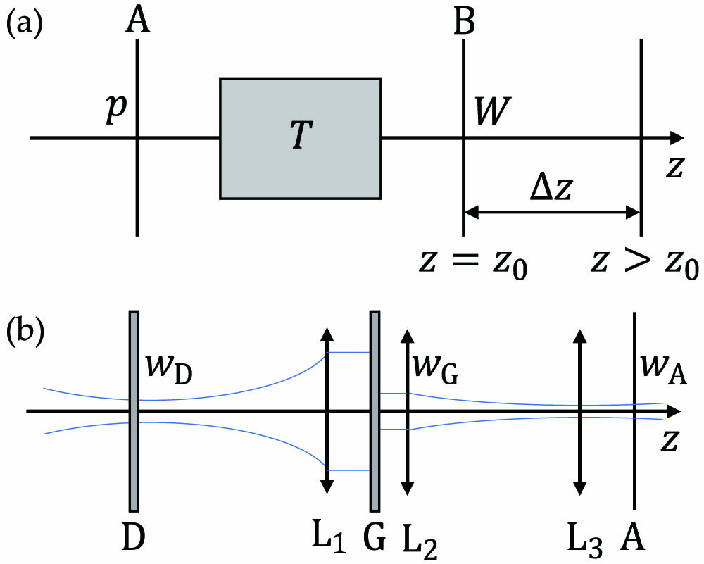
Fig. 1. (a) Experimental setup for transforming a globally incoherent field at plane A into a custom-designed partially coherent beam at plane B using a linear optical transformation system T . (b) Generation of the globally incoherent field at plane A : D is a dynamic diffuser to reduce spatial coherence of the incident focused laser beam, L 1 is a collimating lens, L 2 and L 3 form an afocal imaging system of magnification m ′ = 1 / 5 , G is a Gaussian filter, and the metasurface is placed at plane A . The beam radii at planes D , G , and A are w D , w G , and w A , and the coherence radii at G and B are σ G and σ B .

Fig. 2. Properties of RAP beams of order m = 0 with λ = 633 nm , w 0 = 300 μm , and q = 1 / 30 . (a) Cross sections of the DOC and (b) far-field (at z = 10 z R ) spectral densities when C 0 = − 1 , ρ s → 0 (black), ρ s = 1 (red), ρ s = 2 (green), and ρ s = 4 (blue).

Fig. 3. (a) Operating geometry and design parameters of the Bragg carrier grating. θ is the first Bragg angle of incidence from air to the substrate of refractive index n s and θ ′ from the substrate to the grating layer with refractive index n . h is the groove depth, c is the ridge width, and d is the period. (b) Efficiency η − 1 of order l = − 1 as a function of the fill factor in TE polarization. (c) Efficiency η − 1 as a function of angle of incidence for different fill factors.

Fig. 4. SEM images of a fabricated grating. (a) Side view. (b) Top view.

Fig. 5. Measured absolute value of the spatial DOC μ ( Δ x , z 0 ) (blue) and the spectral density S ( x , z 0 ) (orange) at plane A .

Fig. 6. Spatially varying transmission efficiency η − 1 of the designed metasurface for the RAP beams of order (a) m = 3 and (b) m = 0 .

Fig. 7. Measured and simulated complex degrees of source-plane spatial coherence of the RAP beam with m = 3 (top row) and m = 0 (bottom row). (a)–(d) Absolute values and (e)–(h) phases of μ ( Δ x , Δ y ) . Here, (a), (b), (e), and (f) are the measured results, while (c), (d), (g), and (h) are the simulated results.

Fig. 8. Illustration of propagation characteristics of RAP-beam with m = 3 . The measured intensity profiles at four different propagation distances are in the top row, and the simulation is in the bottom row.

Fig. 9. Same as Fig. 8 but for the beam with m = 0 . The parameters used for the calculations were w 0 = 210 μm , R = 1 / 7.5 , and q = 1 / 30 .

Set citation alerts for the article
Please enter your email address