• Acta Optica Sinica
  • Vol. 41, Issue 1, 0114005 (2021)
Heping Zeng1、2、3、** and Junsong Peng1、2、*
Author Affiliations
  • 1State Key Laboratory of Precision Spectroscopy, East China Normal University, Shanghai 200062, China
  • 2Chongqing Institute, East China Normal University, Chongqing 401120, China
  • 3Jinan Institute of Quantum Technology, Jinan, Shandong 250101, China
  • show less
    DOI: 10.3788/AOS202141.0114005 Cite this Article Set citation alerts
    Heping Zeng, Junsong Peng. Time-Varying Dynamics of Mode-Locked Fiber Lasers[J]. Acta Optica Sinica, 2021, 41(1): 0114005 Copy Citation Text show less
    Build-up of dissipative solitons in laser. (a) Real-time measurement system; (b) different stages during build-up of dissipative soliton
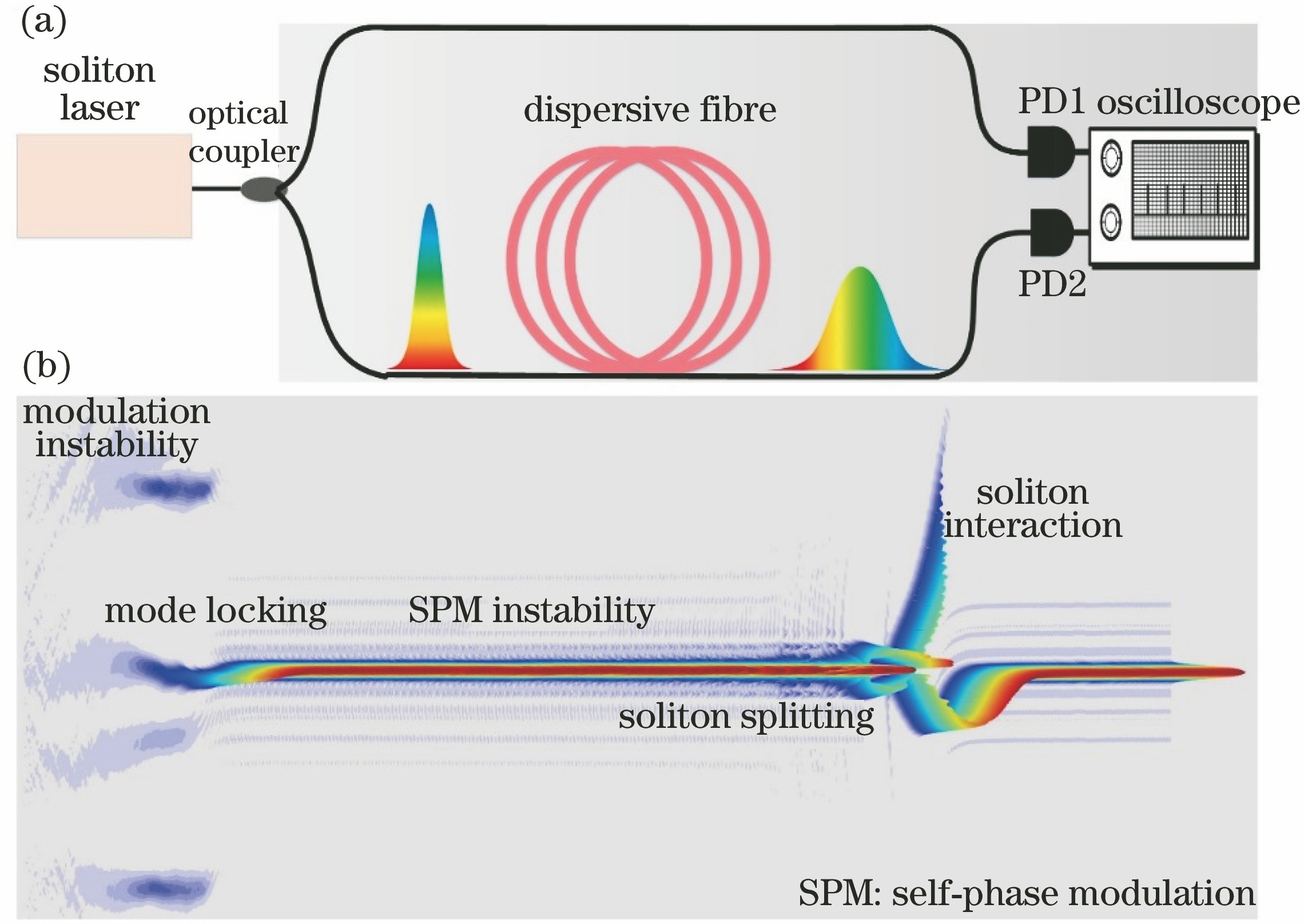
    Fig. 1. Build-up of dissipative solitons in laser. (a) Real-time measurement system; (b) different stages during build-up of dissipative soliton
    Build-up of dissipative solitons for long cavity (16 m) and short cavity (10 m). (a)(b) Spectral evolution during dissipative soliton build-up measured by DFT; (c)(d) field autocorrelation obtained by Fourier transform for spectra
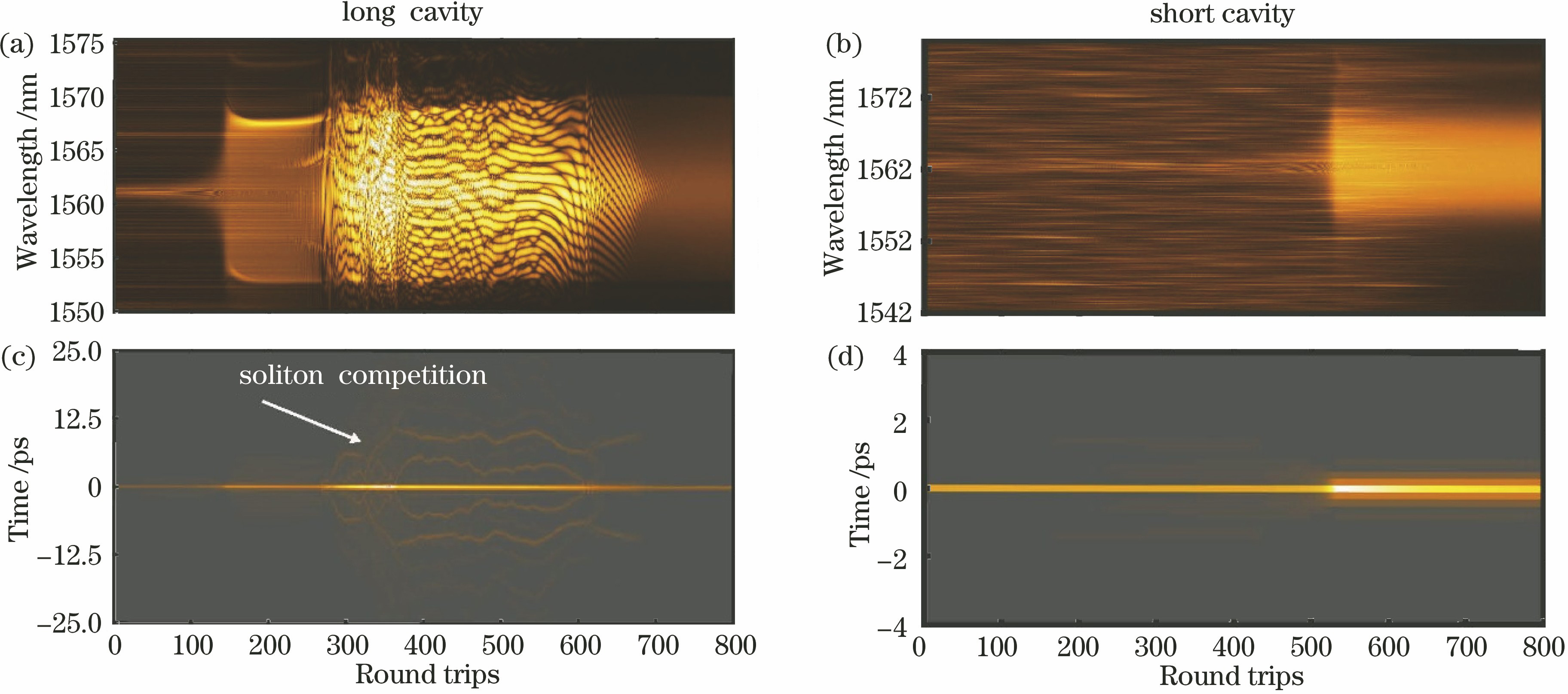
    Fig. 2. Build-up of dissipative solitons for long cavity (16 m) and short cavity (10 m). (a)(b) Spectral evolution during dissipative soliton build-up measured by DFT; (c)(d) field autocorrelation obtained by Fourier transform for spectra
    Build-up of dissipative solitons obtained by simulations[39]. (a) Temporal evolution; (b) autocorrelation evolution; (c) magnified soliton interaction region. Inset is temporal evolution of double solitons
    Fig. 3. Build-up of dissipative solitons obtained by simulations[39]. (a) Temporal evolution; (b) autocorrelation evolution; (c) magnified soliton interaction region. Inset is temporal evolution of double solitons
    Ground-state soliton molecule formation[47]. (a) Real-time spectral evolution measured by DFT (TS-DFT); (b) field autocorrelation traces obtained from TS-DFT; (c)(d) enlargement corresponding to dashed boxes in Fig. 4(b); (e)--(h) repeated measurement results. Results show that the formation dynamics of soliton molecules can be considerably different. Figure 4(b) mainly shows attractive interactions, whereas Figs. 4(f) and 4(h) show vibration and annihilation, respectively. Final soliton molecule is the same, although formation process is different
    Fig. 4. Ground-state soliton molecule formation[47]. (a) Real-time spectral evolution measured by DFT (TS-DFT); (b) field autocorrelation traces obtained from TS-DFT; (c)(d) enlargement corresponding to dashed boxes in Fig. 4(b); (e)--(h) repeated measurement results. Results show that the formation dynamics of soliton molecules can be considerably different. Figure 4(b) mainly shows attractive interactions, whereas Figs. 4(f) and 4(h) show vibration and annihilation, respectively. Final soliton molecule is the same, although formation process is different
    Formation of soliton molecule under excitation state[47]. (a) TS-DFT; (b) field autocorrelation traces corresponding to spectra; (c) spectral and (d) field autocorrelation traces of soliton molecule under stable excitation state
    Fig. 5. Formation of soliton molecule under excitation state[47]. (a) TS-DFT; (b) field autocorrelation traces corresponding to spectra; (c) spectral and (d) field autocorrelation traces of soliton molecule under stable excitation state
    Formations of soliton molecules under ground and excitation states obtained by numerical simulation[47]. (a) Ground state; (b) excitation state
    Fig. 6. Formations of soliton molecules under ground and excitation states obtained by numerical simulation[47]. (a) Ground state; (b) excitation state
    Dynamics of soliton molecule with intermittent vibration. (a) TS-DFT of formation of soliton molecule with intermittent vibration; (b) field autocorrelation traces corresponding to spectra
    Fig. 7. Dynamics of soliton molecule with intermittent vibration. (a) TS-DFT of formation of soliton molecule with intermittent vibration; (b) field autocorrelation traces corresponding to spectra
    Breather in normal dispersion mode-locked laser obtained by experiment[59]. (a)(d)(g) TS-DFT of breather; (b)(e)(h) temporal evolution of breather; (c)(f) widest and narrowest spectra of breather within a period; (i) single-shot spectrum. Net dispersion is 0.14 ps2
    Fig. 8. Breather in normal dispersion mode-locked laser obtained by experiment[59]. (a)(d)(g) TS-DFT of breather; (b)(e)(h) temporal evolution of breather; (c)(f) widest and narrowest spectra of breather within a period; (i) single-shot spectrum. Net dispersion is 0.14 ps2
    Dynamics of breather molecule[59]. (a) TS-DFT of breather molecule; (b) widest and narrowest spectra within a period; (c) temporal evolution of breather molecule; (d) temporal intensity profiles of strongest and weakest breather molecules within a period
    Fig. 9. Dynamics of breather molecule[59]. (a) TS-DFT of breather molecule; (b) widest and narrowest spectra within a period; (c) temporal evolution of breather molecule; (d) temporal intensity profiles of strongest and weakest breather molecules within a period
    Temporal evolution and spectrum of breather obtained by simulation, and temporal evolution and spectrum of dissipative soliton corresponding to traditional mode locking[59]. (a) Spectrum and (b) temporal evolution of breather obtained by simulation; (c) spectrum and (d) temporal evolution of dissipative soliton corresponding to traditional mode locking
    Fig. 10. Temporal evolution and spectrum of breather obtained by simulation, and temporal evolution and spectrum of dissipative soliton corresponding to traditional mode locking[59]. (a) Spectrum and (b) temporal evolution of breather obtained by simulation; (c) spectrum and (d) temporal evolution of dissipative soliton corresponding to traditional mode locking
    Laser output obtained by numerical simulation[60]. (a) Spectrum of stable dissipative solitons from laser; (b) spectral shape of stable dissipative solitons; (c) spectrum exhibits periodic switching among three shapes when increasing pump power further; (d) shapes of three spectra in Fig. 11(c)
    Fig. 11. Laser output obtained by numerical simulation[60]. (a) Spectrum of stable dissipative solitons from laser; (b) spectral shape of stable dissipative solitons; (c) spectrum exhibits periodic switching among three shapes when increasing pump power further; (d) shapes of three spectra in Fig. 11(c)
    Experimentally measured laser output[60]. (a) Spectrum of stable dissipative solitons from laser at pump power of 23.3 mW; (b) spectrum intensity of stable dissipative solitons; (c) spectrum exhibits periodic switching among three shapes when increasing pump power to 28 mW; (d) intensity of three spectra
    Fig. 12. Experimentally measured laser output[60]. (a) Spectrum of stable dissipative solitons from laser at pump power of 23.3 mW; (b) spectrum intensity of stable dissipative solitons; (c) spectrum exhibits periodic switching among three shapes when increasing pump power to 28 mW; (d) intensity of three spectra
    Stable mode-locking and traditional soliton explosion[69]. (a) Spectrum measured under stable mode locking; (b) good agreement between spectra measured by optical spectrum analyzer (OSA) and DFT confirms accuracy of DFT; (c) spectrum of soliton explosion when pump power is 155 mW; (d) spectra of soliton explosion and stable soliton when pump power is 155 mW; (e) spectrum of soliton explosion when pump power is 157 mW; (f) spectra of soliton explosion and stable soliton
    Fig. 13. Stable mode-locking and traditional soliton explosion[69]. (a) Spectrum measured under stable mode locking; (b) good agreement between spectra measured by optical spectrum analyzer (OSA) and DFT confirms accuracy of DFT; (c) spectrum of soliton explosion when pump power is 155 mW; (d) spectra of soliton explosion and stable soliton when pump power is 155 mW; (e) spectrum of soliton explosion when pump power is 157 mW; (f) spectra of soliton explosion and stable soliton
    Soliton collision induced explosions[69]. (a) Temporal evolution of pulse recorded by oscilloscope. White solid line shows energy evolution, inset (top right) is magnified version of small dashed box showing "resurrection" of second pulse; (b) three representative temporal evolutions in Fig. 14(a); (c) real-time spectral evolution measured synchronously by time stretching method; (d) three representative temporal evolutions in Fig. 14(c); (e) magnified portion of dotted box in Fig. 14(d), showing interference pattern
    Fig. 14. Soliton collision induced explosions[69]. (a) Temporal evolution of pulse recorded by oscilloscope. White solid line shows energy evolution, inset (top right) is magnified version of small dashed box showing "resurrection" of second pulse; (b) three representative temporal evolutions in Fig. 14(a); (c) real-time spectral evolution measured synchronously by time stretching method; (d) three representative temporal evolutions in Fig. 14(c); (e) magnified portion of dotted box in Fig. 14(d), showing interference pattern
    Details of soliton collision[69]. (a) Real-time spectral evolution showing interference pattern of double solitons (for a round-trip number from 8500 to 8800) and subsequent chaotic spectrum caused by soliton explosion; white line shows energy evolution; (b) three representative spectral cross-sections at round-trip numbers of 8600, 8850, and 8900, respectively; (c) field autocorrelation traces calculated from spectra; (d) three representative field autocorrelation traces
    Fig. 15. Details of soliton collision[69]. (a) Real-time spectral evolution showing interference pattern of double solitons (for a round-trip number from 8500 to 8800) and subsequent chaotic spectrum caused by soliton explosion; white line shows energy evolution; (b) three representative spectral cross-sections at round-trip numbers of 8600, 8850, and 8900, respectively; (c) field autocorrelation traces calculated from spectra; (d) three representative field autocorrelation traces
    Switching among breather explosion, breather, and continuous wave mode locking by varying pump power
    Fig. 16. Switching among breather explosion, breather, and continuous wave mode locking by varying pump power
    Dynamics of breather explosion[112]. (a) Spectral evolution; (b) five representative spectra in Fig. 17(a), corresponding to round trip numbers of 300, 500, 600, 616, and 620, respectively
    Fig. 17. Dynamics of breather explosion[112]. (a) Spectral evolution; (b) five representative spectra in Fig. 17(a), corresponding to round trip numbers of 300, 500, 600, 616, and 620, respectively
    Heping Zeng, Junsong Peng. Time-Varying Dynamics of Mode-Locked Fiber Lasers[J]. Acta Optica Sinica, 2021, 41(1): 0114005
    Download Citation