• Advanced Photonics
  • Vol. 5, Issue 6, 066004 (2023)
Bingying Zhao1、* and Jerome Mertz2
Author Affiliations
  • 1Boston University, Department of Electrical and Computer Engineering, Boston, Massachusetts, United States
  • 2Boston University, Department of Biomedical Engineering, Boston, Massachusetts, United States
  • show less
    DOI: 10.1117/1.AP.5.6.066004 Cite this Article Set citation alerts
    Bingying Zhao, Jerome Mertz. Resolution enhancement with deblurring by pixel reassignment[J]. Advanced Photonics, 2023, 5(6): 066004 Copy Citation Text show less
    Principle of DPR. (a) From left to right: simulations of Gaussian PSF intensity and gradient maps (amplitude and direction), pixel reassignments, deblurred PSF image after application of DPR. (b) DPR workflow.
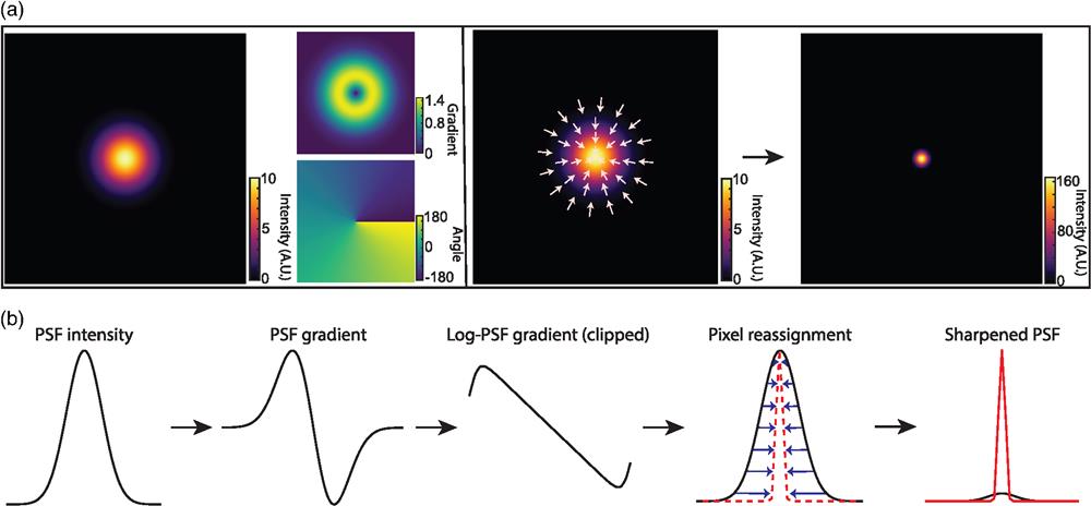
    Fig. 1. Principle of DPR. (a) From left to right: simulations of Gaussian PSF intensity and gradient maps (amplitude and direction), pixel reassignments, deblurred PSF image after application of DPR. (b) DPR workflow.
    DPR resolution enhancement. (a) Simulation of DPR applied to two point objects separated by 1.68σ and 1.41σ. Left, images before (RAW) and after application of DPR gain 1 (DPR1) and DPR gain 2 (DPR2). Right, intensity plots across imaged points. Scale bar, 2σ. (b) DPR applied to fluorescent lines of increasing separation from 0 to 390 nm. Scale bar, 800 nm. PSF FWHM, 4 pixels. Local-minimum filter radius, 7 pixels.
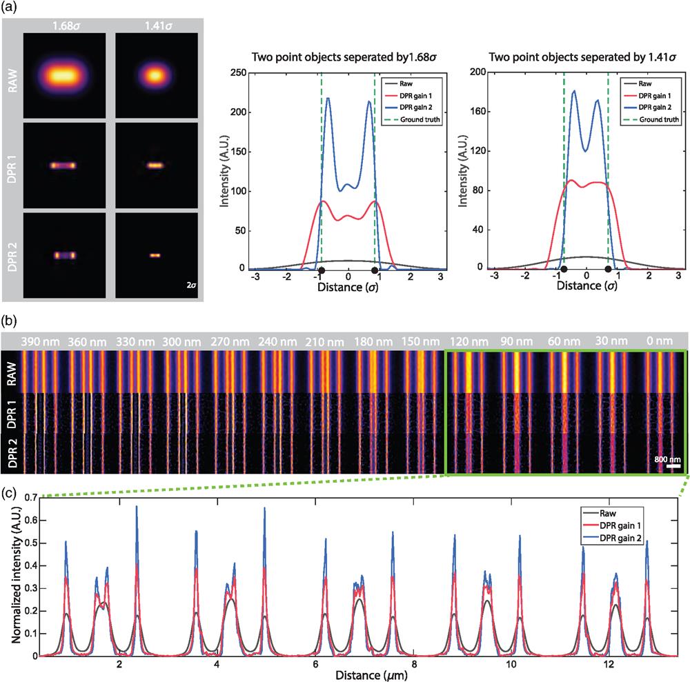
    Fig. 2. DPR resolution enhancement. (a) Simulation of DPR applied to two point objects separated by 1.68σ and 1.41σ. Left, images before (RAW) and after application of DPR gain 1 (DPR1) and DPR gain 2 (DPR2). Right, intensity plots across imaged points. Scale bar, 2σ. (b) DPR applied to fluorescent lines of increasing separation from 0 to 390 nm. Scale bar, 800 nm. PSF FWHM, 4 pixels. Local-minimum filter radius, 7 pixels.
    SMLM Challenge 2016. (a) DPR applied to each frame in raw image stack, followed by temporal mean or variance. (i) Raw image stack, (ii) mean of raw images,, (iii) DPR gain 1 followed by mean, (iv) DPR gain 2 followed by mean, (v) DPR gain 1 followed by variance, and (vi) DPR gain 2 followed by variance. Scale bar, 650 nm. (b) Expanded regions of interest (ROIs) indicated by green square in (a). Bottom left, intensity distribution along red line in ROIs. Bottom right, intensity distribution along green line in ROIs. Scale bar, 200 nm. (c) Image mean followed by DPR. (vii) gain 1, (viii) gain 2. Scale bar, 500 nm. (d) Expanded ROIs indicated by yellow squares in (c) and (ii), (iii), and (iv) in (a). Right, intensity distribution along cyan line in ROIs. Scale bar, 150 nm. PSF FWHM, 2.7 pixels. Local-minimum filter radius, 5 pixels.
    Fig. 3. SMLM Challenge 2016. (a) DPR applied to each frame in raw image stack, followed by temporal mean or variance. (i) Raw image stack, (ii) mean of raw images,, (iii) DPR gain 1 followed by mean, (iv) DPR gain 2 followed by mean, (v) DPR gain 1 followed by variance, and (vi) DPR gain 2 followed by variance. Scale bar, 650 nm. (b) Expanded regions of interest (ROIs) indicated by green square in (a). Bottom left, intensity distribution along red line in ROIs. Bottom right, intensity distribution along green line in ROIs. Scale bar, 200 nm. (c) Image mean followed by DPR. (vii) gain 1, (viii) gain 2. Scale bar, 500 nm. (d) Expanded ROIs indicated by yellow squares in (c) and (ii), (iii), and (iv) in (a). Right, intensity distribution along cyan line in ROIs. Scale bar, 150 nm. PSF FWHM, 2.7 pixels. Local-minimum filter radius, 5 pixels.
    Comparison of DPR, MSSR, and SRRF performances. (a) Images of BPAE cells acquired by a confocal microscope and after DPR gain 2, first order MSSR, and SRRF. DPR parameters: PSF FWHM, 4 pixels; local-minimum filter radius, 12 pixels; DPR gain, 2. MSSR: PSF FWHM, 4 pixels; magnification, 2; order, 1. SRRF: ring radius, 0.5, magnification, 2;, axes, 6. Scale bar, 5 μm. (b) Intensity profiles along single F-actin indicated by red lines in (c). (c) Intensity profiles along proximal F-actin filaments by yellow lines in (a). (d) Expanded ROIs indicated by cyan square in (a). Scale bar, 1.5 μm.
    Fig. 4. Comparison of DPR, MSSR, and SRRF performances. (a) Images of BPAE cells acquired by a confocal microscope and after DPR gain 2, first order MSSR, and SRRF. DPR parameters: PSF FWHM, 4 pixels; local-minimum filter radius, 12 pixels; DPR gain, 2. MSSR: PSF FWHM, 4 pixels; magnification, 2; order, 1. SRRF: ring radius, 0.5, magnification, 2;, axes, 6. Scale bar, 5  μm. (b) Intensity profiles along single F-actin indicated by red lines in (c). (c) Intensity profiles along proximal F-actin filaments by yellow lines in (a). (d) Expanded ROIs indicated by cyan square in (a). Scale bar, 1.5  μm.
    Comparison of DPR, SRRF, and MSSR with optical pixel reassignment and deconvolution. (a) Left, BPAE cells imaged using optical pixel reassignment and deconvolution with Nikon confocal microscope without (top) and with SoRa superresolution enhanced by RL deconvolution (20 iterations). Right, confocal images deblurred by RL deconvolution (20 iterations), DPR (gains 1 and 2), SRRF, and MSSR. DPR parameters: PSF FWHM, 2 pixels; local-minimum filter radius, 40 pixels. MSSR parameters: PSF FWHM, 2 pixels; magnification, 4; order, 1. SRRF: ring radius, 0.5; magnification, 4; axes, 6. Scale bar, 2 μm. (b) Zoom-in ROIs indicated by red squares in (a). Scale bar, 600 nm.
    Fig. 5. Comparison of DPR, SRRF, and MSSR with optical pixel reassignment and deconvolution. (a) Left, BPAE cells imaged using optical pixel reassignment and deconvolution with Nikon confocal microscope without (top) and with SoRa superresolution enhanced by RL deconvolution (20 iterations). Right, confocal images deblurred by RL deconvolution (20 iterations), DPR (gains 1 and 2), SRRF, and MSSR. DPR parameters: PSF FWHM, 2 pixels; local-minimum filter radius, 40 pixels. MSSR parameters: PSF FWHM, 2 pixels; magnification, 4; order, 1. SRRF: ring radius, 0.5; magnification, 4; axes, 6. Scale bar, 2  μm. (b) Zoom-in ROIs indicated by red squares in (a). Scale bar, 600 nm.
    Engineered cardiac tissue imaging. (a) DPR gain 1 applied to simulated ground-truth wide-field images of monolayer hiPSC-CMs derived from experimental images acquired by a confocal microscope. Left, simulated ground truth. Middle, simulated wide-field intensity image without (top) and with (bottom) application of DPR, and corresponding error maps. Right, intensity profile along sarcomere chain indicated by the cyan rectangle. PSF FWHM, 4 pixels; local-minimum filter radius, 7 pixels. (b) DPR gain 1 applied to experimental low-resolution images of hiPSC-CMTs. Left, confocal image. Middle, DPR-enhanced image. Right, intensity profile of sarcomere chain indicated by the red rectangle. PSF FWHM, 4 pixels; local-minimum filter radius, 7 pixels. (c) DPR gain 1 applied to experimental high-resolution images of hiPSC-CMT. Left, confocal image. Middle, DPR-enhanced image. Right, intensity profile of the sarcomere chain indicated by the yellow rectangle. PSF FWHM, 2 pixels; local-minimum filter radius, 4 pixels. Scale bar, 15 μm.
    Fig. 6. Engineered cardiac tissue imaging. (a) DPR gain 1 applied to simulated ground-truth wide-field images of monolayer hiPSC-CMs derived from experimental images acquired by a confocal microscope. Left, simulated ground truth. Middle, simulated wide-field intensity image without (top) and with (bottom) application of DPR, and corresponding error maps. Right, intensity profile along sarcomere chain indicated by the cyan rectangle. PSF FWHM, 4 pixels; local-minimum filter radius, 7 pixels. (b) DPR gain 1 applied to experimental low-resolution images of hiPSC-CMTs. Left, confocal image. Middle, DPR-enhanced image. Right, intensity profile of sarcomere chain indicated by the red rectangle. PSF FWHM, 4 pixels; local-minimum filter radius, 7 pixels. (c) DPR gain 1 applied to experimental high-resolution images of hiPSC-CMT. Left, confocal image. Middle, DPR-enhanced image. Right, intensity profile of the sarcomere chain indicated by the yellow rectangle. PSF FWHM, 2 pixels; local-minimum filter radius, 4 pixels. Scale bar, 15  μm.
    Multi-z confocal zebrafish imaging. (a) In vivo raw and DPR-enhanced (gain 1) multiplane images of the brain region in a zebrafish 9 dpf. Left, four image planes. Right, merged with colors corresponding to depth. ROIs indicated by the red and yellow rectangles in (a) are shown in Fig. S8 in the Supplementary Material. Scale bar, 25 μm. (b) Raw and DPR-enhanced multiplane images of the zebrafish tail region. Scale bar, 25 μm. (c) ROI indicated by the cyan rectangle in (b), and intensity profile along the cyan dashed line. ROI indicated by the magenta rectangle in (b) is shown in Fig. S8 in the Supplementary Material. Scale bar, 10 μm. (d) Merged multiplane images in the tail region of a zebrafish. Left, raw low-resolution multiplane image. Middle, DPR-enhanced low-resolution multiplane image. Right, raw high-resolution multiplane image (different fish and tail regions). PSF FWHM, 5 pixels; local-minimum filter radius, 25 pixels. Scale bar, 20 μm. Planes 1 to 4, the deepest to the shallowest. Interplane separation, 20 μm.
    Fig. 7. Multi-z confocal zebrafish imaging. (a) In vivo raw and DPR-enhanced (gain 1) multiplane images of the brain region in a zebrafish 9 dpf. Left, four image planes. Right, merged with colors corresponding to depth. ROIs indicated by the red and yellow rectangles in (a) are shown in Fig. S8 in the Supplementary Material. Scale bar, 25  μm. (b) Raw and DPR-enhanced multiplane images of the zebrafish tail region. Scale bar, 25  μm. (c) ROI indicated by the cyan rectangle in (b), and intensity profile along the cyan dashed line. ROI indicated by the magenta rectangle in (b) is shown in Fig. S8 in the Supplementary Material. Scale bar, 10  μm. (d) Merged multiplane images in the tail region of a zebrafish. Left, raw low-resolution multiplane image. Middle, DPR-enhanced low-resolution multiplane image. Right, raw high-resolution multiplane image (different fish and tail regions). PSF FWHM, 5 pixels; local-minimum filter radius, 25 pixels. Scale bar, 20  μm. Planes 1 to 4, the deepest to the shallowest. Interplane separation, 20  μm.
    Bingying Zhao, Jerome Mertz. Resolution enhancement with deblurring by pixel reassignment[J]. Advanced Photonics, 2023, 5(6): 066004
    Download Citation