Ionization balance of non-LTE plasmas from an average-atom collisional-radiative model

A. A. Ovechkin; P. A. Loboda; A. S. Korolev; S. V. Kolchugin; I. Yu. Vichev; A. D. Solomyannaya; D. A. Kim; A. S. Grushin

doi:10.1063/5.0098814

Abstract

We present a simplified version of an average-atom collisional-radiative model employing both local-thermodynamic-equilibrium average-atom and isolated-ion atomic data. The simplifications introduced do not lead to any substantial errors, and they significantly speed up calculations compared with the basic average-atom model involving direct solution of the self-consistent-field equations. Average ion charges, charge state distributions, and emission spectra of non-local-thermodynamic-equilibrium (NLTE) gold plasmas calculated using various modifications of the average-atom collisional-radiative model are compared with those obtained using the THERMOS model with the detailed configuration accounting approach. We also propose an efficient method to calculate thermodynamic functions of NLTE plasmas in the context of the simplified average-atom collisional-radiative model.

Ionization balance of non-local-thermodynamic-equilibrium (NLTE) plasmas is generally calculated using collisional–radiative models that enable one to represent plasma particle-to-particle and particle-to-radiation interactions at various levels of detail. Most of these models are based on the chemical-picture approach which deals with plasma ions in various quantum states and free electrons1 so that relative populations of detailed ion states or some sets of these (e.g., electronic configurations or superconfigurations1,2) are related to each other by rate equations. To solve these equations, one needs first to generate consistent datasets of the relevant energy levels and atomic-process rates.

In principle, the ionization balance of NLTE plasmas along with their radiative and thermodynamic properties might be accurately represented through a detailed ion-state accounting approach. However, in hot plasmas, even the number of essentially populated electronic configurations frequently appears to be so large that NLTE radiation-hydrodynamics modeling becomes prohibitively expensive. In such cases, one can employ a collisional-radiative model for the sets of electronic configurations with close average energies, i.e., superconfigurations,1,3–6 which provides the possibility to considerably reduce computational cost without noticeable loss of accuracy. The use of a superconfiguration collisional–radiative model, however, faces an additional difficulty stemming from the need to evaluate the effective temperatures responsible for the energy distribution of electronic configurations within superconfigurations.1,7–10 On the other hand, some averaged account of bound-electron structure may be obtained on the basis of a screened-hydrogenic model characterizing electronic shells solely by their principal quantum numbers.11 Although this model enables one to significantly reduce computational cost, it does not provide any way to give a detailed description of radiative properties.

In many applications, detailed knowledge of fractional ionic abundances is not necessary, and one can therefore restrict consideration to the calculation of averaged quantities (average electron-shell occupation numbers and average ion charges) in the context of the average-atom approach.12,13 Most NLTE average-atom models employ the screened-hydrogenic formulation, either including14 or ignoring11 the one-electron energy dependence on the orbital quantum numbers. In these models, electron energies are found in an effective Coulomb potential allowing for outer-shell screening. The charge of this potential is specific to each individual atomic shell and depends on the screening of the nuclear Coulomb potential by the inner-shell electrons. Such models are very inexpensive computationally and are therefore routinely used in radiation-hydrodynamics modeling.15 In the present work, however, we deal with alternative average-atom models16–18 in which one-electron energies and wavefunctions are found from numerical solution of the Schrödinger or Dirac equation with self-consistent-field (SCF) potentials. These models enable one to provide more realistic descriptions of material properties than the screened-hydrogenic models—specifically because of their consistent treatment of plasma density effects, which are automatically included at the stage of solution of the SCF equations in an electrically neutral atomic cell. Nevertheless, for radiation-hydrodynamics modeling, solution of the SCF equations with the NLTE electron-shell occupation numbers repeated over and over again for different values of free-electron temperature and material density would present a formidable task. Therefore, we have developed a simplified, much more tractable, version of the NLTE average-atom model, described in Sec. II.

This NLTE average-atom model is implemented in the RESEOS code19,20 originally developed to calculate thermodynamic and optical properties of LTE plasmas on the basis of the Liberman21 and neutral Wigner–Seitz sphere22 models along with a generalized version19 of the superconfiguration approach.2,23 In Sec. III, the average ion charges, charge-state distributions, and emission spectra of NLTE gold plasmas calculated with RESEOS are compared with those ones obtained using the THERMOS code18,24,25 utilizing the detailed configuration accounting approach and with experimental data.26,27 Section IV describes an efficient and reasonably accurate method for calculating the electron components of the pressure and internal energy of NLTE plasmas.

In the average-atom collisional-radiative model,12,13,16,17 one needs to solve the rate equations for average occupation numbers of electron shells. In the steady-state approximation, these equations take the form $- N_{m} L_{m} + (g_{m} - N_{m}) S_{m} = 0,$ (1)where N_m is the average occupation number of subshell (relativistic shell) m characterized by the set of quantum numbers n_m, l_m, j_m (standing for the principal quantum number and the one-electron orbital and total angular momenta, respectively) and its degeneracy g_m = 2j_m + 1. In Eq. (1), the sink (L_m) and source (S_m) terms represent the total rates of atomic processes respectively depopulating and populating the mth subshell: $L_{m} = \sum_{k} (R_{m k}^{(c)} + R_{m k}^{(r)}) (1 - N_{k} / g_{k}) + R_{m c}^{(c)} + R_{m c}^{(r)} + A_{m},$ (2) $S_{m} = \frac{1}{g_{m}} \sum_{k} (R_{k m}^{(c)} + R_{k m}^{(r)}) N_{k} + R_{c m}^{(c)} + R_{c m}^{(r)} + D_{m},$ (3)where A_m and D_m are the autoionization and dielectronic capture rates, respectively. Subscripts a and b in the notation for the atomic-process rates $R_{a b}^{(c, r)}$ refer to the electron subshells m and k or the continuum state c involved in the relevant one-electron transition a → b, while the superscripts correspond to the type of atomic process—collisional (c) or radiative (r).

Note that in the non-steady-state situations encountered in hydrodynamics simulations, the right-hand side of Eq. (1) becomes dN_m/dt, which can be readily approximated by some finite-difference formula and even improves the convergence of iterations for obtaining occupation numbers (which may be coupled with iterations to obtain the radiation field and free-electron temperature) at the running time step. In the present paper, we deal only with the steady-state cases and therefore omit the term dN_m/dt.

Below, we present detailed expressions for the atomic-process rates employed in RESEOS.

For collisional excitation, we account only for the dipole transitions k → m with |l_k − l_m| = 1 and $| j_{k} - j_{m} | ⩽ 1$ , and we use an expression for the rate $R_{k m}^{(c)}$ (ɛ_k < ɛ_m) that is applicable in both the limits of large and small free-electron energies: $R_{k m}^{(c)} = \frac{4 \sqrt{2 π β} e^{4} Z_{0} n_{i}^{0} f_{k m}}{\sqrt{m_{e}} ε_{k m}} Λ (β ε_{k m}),$ (4) $\begin{align} Λ (x) & = \exp (- x) [\exp (x) E_{1} (x) + \frac{π a}{\sqrt{3}}] \\ \approx \exp (- x) \ln [\frac{1}{\exp (γ) x} + \exp (\frac{π a}{\sqrt{3}})] . \end{align}$ (5)Here, e is the elementary charge, m_e is the electron mass, and Z₀ is the average ion charge (in units of e), defined as the difference between the nuclear charge Z (also in units of e) and the number of bound electrons: $Z_{0} = Z - \sum_{m} N_{m},$ (6)ɛ_j is the one-electron energy relevant to subshell j, ɛ_km = ɛ_m − ɛ_k, β = 1/T_e, with T_e being the free-electron temperature (in energy units), $n_{i}^{0}$ is the ion density, $E_{1} (x) = \int_{x}^{\infty} \exp (- t) d t / t$ , γ = 0.5772 … is the Euler–Mascheroni constant, and f_km is the oscillator strength of the one-electron transition k → m. The parameter a in Eq. (5) is set to 0.2 to provide the threshold value of the excitation cross-section approximating the results of benchmark calculations for positive ions in the distorted-wave approximation.28 This value of a would be incorrect for neutral atoms,28 but this is not the case here since the present average-atom model itself does not work at temperatures so low that neutral atoms could exist.

To derive Eqs. (4) and (5), one should consider only binary electron–ion collisions and assume that at sufficiently large energies ɛ of the incident electron (compared with ɛ_km), the momentum q transferred to the ion is constrained within the limits29 $\begin{gathered} q_{\min} = \sqrt{2 m_{e} ε} - \sqrt{2 m_{e} (ε - ε_{k m})} \approx \sqrt{m_{e}} ε_{k m} / \sqrt{2 ε}, \\ q_{\max} = \sqrt{2 m_{e} ε} + \sqrt{2 m_{e} (ε - ε_{k m})} \approx 2 \sqrt{2 m_{e} ε} . \end{gathered}$ (7)An additional restriction on the momentum q follows from the validity condition for the binary-collision approximation (see Ref. 30):31q ≳ ℏ/d, where ℏ is the reduced Planck constant and d is the characteristic range of localization of the plasma-ion potential, $d = \max (r_{0}, r_{De}),$ (8)with $r_{0} = {[3 / (4 π n_{i}^{0})]}^{1 / 3}$ and r_De the electron Debye radius. Using the fact that ɛ ∼ 1/β, the relevant restriction on the argument of the Coulomb logarithm Λ(βɛ_km) takes the form $q_{\max} / q_{\min} \sim \sqrt{m_{e} ε} / q_{\min} \sim ε / ε_{k m} \sim 1 / (β ε_{k m}) ≲ \sqrt{m_{e}} d / (ℏ \sqrt{β})$ . Therefore, in the case $β ε_{k m} < ℏ \sqrt{β} / (\sqrt{m_{e}} d)$ , we replace the argument of the Coulomb logarithm βɛ_km by $ℏ \sqrt{β} / (\sqrt{m_{e}} d)$ . This enables us to avoid unphysically large values of the collisional excitation rates in the case of very small transition energies.

The collisional deexcitation rate follows from the known principle of detailed balance: $g_{m} R_{m k}^{(c)} = g_{k} e^{β ε_{k m}} R_{k m}^{(c)} .$ (9)

The collisional ionization rate is calculated using the modified Lotz formula:16,32 $R_{m c}^{(c)} = \frac{2 K \sqrt{2 π β} e^{4} Z_{0} n_{i}^{0}}{π \sqrt{m_{e}} | ε_{m} |} E_{1} (\max (β | ε_{m} |, \frac{ℏ \sqrt{β}}{\sqrt{m_{e}} d})),$ (10)where K = 2.27.16 The three-body recombination rate is connected with the collisional ionization rate by the principle of detailed balance (see Ref. 33): $R_{c m}^{(c)} = \exp [β (μ_{e} - ε_{m})] R_{m c}^{(c)},$ (11)where μ_e is the chemical potential of free electrons.

For sufficiently narrow profiles of absorption/emission lines, the rate of radiative excitation/deexcitation may be written as (see, e.g., Ref. 1) $R_{k m}^{(r)} = \frac{2 e^{2}}{ℏ^{2} m_{e} c^{3}} ε_{k m}^{2} | f_{k m} | [θ (ε_{m k}) + F (| ε_{k m} |)] .$ (12)Here, c is the speed of light, θ(x) is the Heaviside function, and $F (ω) = \frac{1}{4 π} \int f (ω, Ω) d Ω$ (13)with f(ω,Ω) being the distribution function of photons with energy ω and a specific polarization relative to the dimensionless phase-space unit volume drdp/(2πℏ)³. The function (13) is readily expressed in terms of the radiation-energy spectral density U(ω) as F(ω) = π²(ℏc)³U(ω)/ω³.

The photoionization $(R_{m c}^{(r)})$ and photorecombination $(R_{c m}^{(r)})$ rates are evaluated in a similar way: $R_{m c}^{(r)} = \frac{2 e^{2}}{ℏ^{2} m_{e} c^{3}} \int_{| ε_{m} |}^{\infty} ω^{2} f_{m} (ε_{m} + ω) [1 - n (ε_{m} + ω)] F (ω) d ω,$ (14) $\begin{align} R_{c m}^{(r)} & = \exp [β (μ_{e} - ε_{m})] \frac{2 e^{2}}{ℏ^{2} m_{e} c^{3}} \int_{| ε_{m} |}^{\infty} ω^{2} f_{m} (ε_{m} + ω) \\ \times [1 - n (ε_{m} + ω)] \exp (- β ω) [1 + F (ω)] d ω, \end{align}$ (15)where n(ɛ) is the Fermi–Dirac distribution $n (ε) = \frac{1}{1 + \exp [β (ε - μ_{e})]} .$ (16)

The bound–free oscillator strength f_m(ɛ) can be calculated in the distorted-wave approximation with the numerical wavefunctions found in an SCF potential (e.g., an average-atom or isolated-ion potential): $\begin{align} f_{m} (ε) & = \frac{m_{e} (ε - ε_{m})}{3 ℏ^{2}} \sum_{l_{c} = l_{m} \pm 1, j_{c}} \frac{2 j_{c} + 1}{j_{m} + j_{c} + 1} \\ \times [δ_{| j_{m} - j_{c} |, 1} + δ_{| j_{m} - j_{c} |, 0} \frac{2}{(2 l_{m} + 1) (2 l_{c} + 1)}] r_{m, ε l_{c} j_{c}}^{2}, \end{align}$ (17) $r_{m, ε l_{c} j_{c}} = \int_{0}^{\infty} r [P_{m} (r) P_{ε l_{c} j_{c}} (r) + Q_{m} (r) Q_{ε l_{c} j_{c}} (r)] d r,$ (18)where δ_ab is the Kronecker delta, and P(r)/r and Q(r)/r are the major and the minor radial components of an electron wavefunction, respectively. An alternative simplified approach to evaluate f_m(ɛ) for multielectron ions is to formally generalize the Kramers formula for hydrogen-like ions (see, e.g., Ref. 34) using its well-known representations $f_{m} (ε) = \frac{4 m_{e}^{2} e^{8} Z_{m}^{4}}{3 \sqrt{3} π ℏ^{4} n_{m}^{5} {(ε - ε_{m})}^{3}}$ (19)and $f_{m} (ε) = \frac{8 \sqrt{2 m_{e}} e^{2} Z_{m} {|ε_{m}|}^{3 / 2}}{3 \sqrt{3} π ℏ n_{m}^{2} {(ε - ε_{m})}^{3}} .$ (20)An effective screened nuclear charge Z_m “seen” by the electrons occupying subshell m is evaluated with More’s screening matrix σ_nr:11 $Z_{m} \equiv Z_{n_{m}} = Z - \sum_{n < n_{m}} σ_{n_{m} n} G_{n} - \frac{1}{2} σ_{n_{m} n_{m}} G_{n_{m}},$ (21)where $G_{n} = \sum_{n_{j} = n} N_{j}$ is the total occupation number of all subshells with the same principal quantum number n. In general, Eqs. (19) and (20) yield different values—the results coinciding only when $| ε_{m} | = m_{e} e^{4} Z_{m}^{2} / (2 ℏ^{2} n_{m}^{2})$ , i.e., for nonrelativistic hydrogen-like ions. In the case of multielectron ions, however, this condition cannot be met even in the context of the screened-hydrogenic model, owing to the disregard of the screening from the outer-shell electrons.11

The autoionization rate A_m in Eq. (2) is found as the net rate of one-electron transitions m → c from subshell m to the continuum occurring simultaneously with all possible bound–bound one-electron transitions j → i from upper subshells j to lower ones i:35 $A_{m} = \sum_{j i} N_{j} (g_{i} - N_{i}) A_{j i}^{m c} θ (ε_{j} - ε_{i} + ε_{m}) .$ (22)Taking into account only dipole transitions with |l_i − l_j| = 1, $| j_{i} - j_{j} | ⩽ 1$ , |l_m − l_c| = 1, and $| j_{m} - j_{c} | ⩽ 1$ , disregarding the exchange terms, and assuming the wavefunction at the inner subshell i to be localized in a much smaller volume than that at the upper subshell m, we get the following expression for the rate $A_{j i}^{m c}$ (see Ref. 13): $A_{j i}^{m c} = \frac{3 π ε_{i j}^{2} f_{i j}}{2 g_{j} ℏ Z_{m}^{2}} f_{m} (ε) (1 - n (ε)) |_{ε = ε_{j} - ε_{i} + ε_{m}} .$ (23)Equation (23) also implies that the electron potential in the peak region of the m-subshell radial wavefunction may be approximated by the Coulomb potential with screening from the outer electrons: $V (r) \approx - \frac{Z_{m} e^{2}}{r} + const .$ (24)In line with this assumption, it would be appropriate to calculate bound–free oscillator strengths f_m(ɛ) using hydrogen-like wavefunctions, corresponding to the potential (24).18 In practice, however, it frequently appears reasonable enough to evaluate bound–free oscillator strengths with the Kramers formula or just to use available oscillator-strength data precalculated in the distorted-wave approximation, since the ionization balance is generally not too sensitive to minor inaccuracies in the oscillator strengths entering Eq. (23).

The rate of the inverse process, i.e., dielectronic capture, reads $D_{m} = \sum_{j i} (g_{j} - N_{j}) N_{i} A_{i j}^{c m} θ (ε_{j} - ε_{i} + ε_{m}),$ (25)where the relevant partial rate $A_{i j}^{c m}$ is connected with $A_{j i}^{m c}$ by the principle of detailed balance (see Refs. 13 and 33): $A_{i j}^{c m} = \exp [β (μ_{e} - ε_{j} + ε_{i} - ε_{m})] A_{j i}^{m c} .$ (26)

Note that Eqs. (14), (15), and (23) contain the free-electron Pauli blocking factor 1 − n(ɛ). In principle, it would be appropriate to include a similar factor in the calculation of the collisional ionization and three-body recombination rates. However, keeping in mind that free-electron degeneracy effects are generally insignificant in high-temperature plasmas under strong NLTE conditions, we use here the simple Lotz formula (10), disregarding the Pauli blocking factor but enabling us to rapidly evaluate the relevant atomic-process rates which is crucial for NLTE simulations.

The variation of NLTE one-electron energies in the process of iterative solution of Eq. (1) may lead to sudden changes in the Heaviside function θ(ɛ_j − ɛ_i + ɛ_m) in Eqs. (22) and (25), thus impeding the convergence of iterations. To improve convergence, we introduce some minor broadening of the two-electron-process thresholds effectively responsible for statistical averaging of one-electron energies over all possible electronic configurations occurring in a plasma. We represent the probability of finding a free electron coming from the m-subshell autoionization with an energy ɛ by a Gaussian function centered at the average energy ⟨ɛ⟩ = ɛ_j − ɛ_i + ɛ_m: $P (ε) = \frac{1}{\sqrt{2 π} Δ} \exp [- \frac{1}{2} {(\frac{ε - ⟨ ε ⟩}{Δ})}^{2}] .$ (27)The Heaviside function θ(ɛ_j − ɛ_i + ɛ_m) in Eqs. (22) and (25) is then replaced by the probability that the autoionization process just leads to the ejection of an electron with positive energy: $\int_{0}^{\infty} P (ε) d ε = \frac{1}{2} [1 + erf (\frac{ε_{j} - ε_{i} + ε_{m}}{\sqrt{2} Δ})],$ (28)where $erf (x) = 2 \int_{0}^{x} \exp (- t^{2}) d t / \sqrt{π}$ is the error function. As Δ approaches zero, Eq. (28) becomes θ(ɛ_j − ɛ_i + ɛ_m). In the present work, rigorous substantiation of the two-electron-process threshold broadening is not performed, and therefore formal expressions for Δ are not derived. Instead, we use ad hoc values of Δ that are large enough to ensure convergence of iterations while being small enough (Δ ≲ 10⁻²T_e) to make the solution of Eq. (1) insensitive to their specific values.

As the calculation of one-electron energies and atomic-process rates is generally rather laborious, Eq. (1) is solved by making two iteration cycles.18 In the internal cycle, one solves the equations for occupation numbers with certain values of one-electron energies, rates of atomic processes, and average ion charge by using the Newton method.36 Note that the convergence of the Newton iterations is both fast and stable, regardless of the local radiation field, provided that the variation of occupation numbers is constrained by the obvious condition $0 ⩽ N_{m} ⩽ g_{m}$ .

In the lth external iteration, the occupation numbers ${\bar{N}}_{p}^{(l)}$ obtained from internal iterations are mixed with those from the preceding (l − 1)th external iteration (see Refs. 18 and 37): $N_{p}^{(l)} = α {\bar{N}}_{p}^{(l)} + (1 - α) N_{p}^{(l - 1)} .$ (29)In the calculations in the present paper, the mixing parameter α is set equal to 0.3. This mixing procedure enables us to considerably improve convergence. Then, the resulting occupation numbers $N_{p}^{(l)}$ are employed in the external iteration to update the values of average ion charge (6), chemical potential μ_e, one-electron energies, and process rates. For the latter procedure, two methods have been implemented. The first (denoted as method I) involves solution of the SCF equations employing a fixed set of (generally noninteger) occupation numbers N_s at given values of free-electron temperature and material density. In the present work, bound electrons are treated with the relativistic Dirac equation, while free ones are represented under the nonrelativistic semiclassical approximation. The corresponding SCF equations thus take the form18,21,38 $P_{s}^{'} (r) + \frac{ϰ_{s}}{r} P_{s} (r) = \frac{1}{ℏ c} [ε_{s} - V (r) + 2 m_{e} c^{2}] Q_{s} (r),$ (30) $Q_{s}^{'} (r) - \frac{ϰ_{s}}{r} Q_{s} (r) = - \frac{1}{ℏ c} [ε_{s} - V (r)] P_{s} (r),$ (31) $V (r) = [V_{el} (r) + V_{xc} (n_{e} (r), β) - V_{xc} (n_{e}^{0}, β) - ν] θ (r_{0} - r),$ (32) $V_{el} (r) = - \frac{Z e^{2}}{r} + 4 π e^{2} \int_{0}^{r_{0}} \frac{{(r^{'})}^{2} n_{e} (r^{'}) d r^{'}}{r_{>}},$ (33) $4 π r^{2} n_{e} (r) = 4 π r^{2} [n_{e}^{(1)} (r) + n_{e, f} (r)] θ (r_{0} - r) + 4 π r^{2} n_{e}^{0} θ (r - r_{0}),$ (34) $4 π r^{2} n_{e}^{(1)} (r) = \sum_{s} N_{s} [P_{s}^{2} (r) + Q_{s}^{2} (r)],$ (35) $n_{e, f} (r) = \frac{\sqrt{2} m_{e}^{3 / 2}}{π^{2} ℏ^{3} β^{3 / 2}} \int_{- β V (r)}^{\infty} \frac{\sqrt{y} d y}{1 + \exp {y + β [V (r) - μ_{e}]}},$ (36) $n_{e}^{0} = n_{e, f} (r > r_{0}),$ (37) $\begin{align} ν & = \frac{1}{n_{e} (r_{0})} \{- n_{e}^{0} ε_{xc} (n_{e}^{0}, β) - [n_{e} (r_{0}) - n_{e}^{0}] V_{xc} (n_{e}^{0}, β) \\ + n_{e} (r_{0}) ε_{xc} (n_{e} (r_{0}), β)\}, \end{align}$ (38) $4 π \int_{0}^{r_{0}} n_{e} (r) r^{2} d r = Z .$ (39)Here, r_> = max(r, r′), ϰ_s = (l_s − j_s)(2j_s + 1), V(r) is the total SCF potential, and V_xc is the exchange-correlation potential found from the exchange-correlation Helmholtz free energy per electron ɛ_xc(n_e, β) through the relation $V_{xc} (n_{e}, β) = \frac{\partial}{\partial n_{e}} [n_{e} ε_{xc} (n_{e},)] .$ (40)The calculations in the present work are carried out with the simple Kohn–Sham exchange potential $V_{xc} (n_{e}) = V_{x} (n_{e}) = - e^{2} {(3 n_{e} / π)}^{1 / 3}$ , which ignores electron correlation effects, which are insignificant at the high temperatures considered in this paper.

The chemical potential is found from the charge-neutrality condition (39).

One-electron energies and wavefunctions obtained from Eqs. (30)–(39) are employed to calculate the oscillator strengths and rates of atomic processes. Since Eqs. (30)–(39) are nonlinear, their solution uses an iterative procedure. In doing this, the potential V(r) is updated in each iteration with the generalized Anderson method,37,39 enabling one to strongly accelerate convergence. The system of Dirac Eqs. (30) and (31) is solved with the phase method,18 which ensures very rapid convergence of iterations for one-electron energies. However, the solution of Eqs. (30)–(39) in every external iteration for Eq. (1) is still very time-consuming. We have therefore developed a second, simplified, perturbation-theory approach referred to as method II. In this method, the SCF Eqs. (30)–(39) are solved only once in the LTE approximation, which assumes that Fermi–Dirac statistics (16) hold: $N_{s} = {\tilde{N}}_{s} = g_{s} n (ε_{s})$ . The results of these LTE calculations are then employed for an approximate evaluation of one-electron energies and atomic-process rates corresponding to the NLTE occupation numbers in the following way.

From Eqs. (30)–(35), one readily finds the relation $ε_{s} w_{s} = (⟨ s ⟩ - ν) w_{s} + e^{2} \sum_{t} N_{t} F_{s t}^{(0)} + Δ I_{s} + Δ ε_{s}^{xc},$ (41)where $w_{s} = \int_{0}^{r_{0}} ρ_{s} (r) d r, with ρ_{s} (r) = P_{s}^{2} (r) + Q_{s}^{2} (r),$ (42) $Δ I_{s} = 4 π e^{2} \int_{0}^{r_{0}} ρ_{s} (r) d r \int_{0}^{r_{0}} \frac{n_{e, f} (r^{'}) {(r^{'})}^{2}}{r_{>}} d r^{'},$ (43) $Δ ε_{s}^{xc} = \int_{0}^{r_{0}} [V_{xc} (n_{e} (r), β) - V_{xc} (n_{e}^{0}, β)] ρ_{s} (r) d r,$ (44) $F_{s t}^{(0)}$ is the zero-rank direct Slater integral: $F_{s t}^{(0)} = \int_{0}^{r_{0}} ρ_{s} (r) d r \int_{0}^{r_{0}} \frac{ρ_{t} (r^{'})}{r_{>}} d r^{'},$ (45)and ⟨s⟩ stands for the sum of the kinetic energy of an electron at subshell s and the potential energy of its interaction with the central nucleus (see, e.g., Ref. 40).

At relatively low material densities, where NLTE effects are expected to be important, one can safely assume that bound-electron wavefunctions are localized inside the atomic cell of radius r₀, and therefore w_s ≈ 1 and ν ≈ 0. We then note that small variations of the occupation numbers entail only slight alterations of the wavefunctions given by the solution of Eqs. (30)–(39). Keeping in mind also that the exchange-correlation contribution (44) to the one-electron energy is generally small compared with the kinetic and electrostatic energy contributions and that the alteration of the potential V_xc(n_e(r), β) in Eq. (44) due to the variation of the occupation numbers is partially counterbalanced by the corresponding alteration of the term $V_{xc} (n_{e}^{0}, β)$ , we can represent the energy (41) as $ε_{s} = ε_{s}^{(0)} + e^{2} \sum_{t} N_{t} F_{s t}^{(0)} + Δ I_{s},$ (46)with the term $ε_{s}^{(0)}$ and the Slater integrals $F_{s t}^{(0)}$ being weakly dependent on the occupation numbers.

The quantity ΔI_s(43) represents the lowering of the ionization potential for an ion at finite material density compared with an isolated ion with the same occupation numbers of electron subshells. To estimate ΔI_s, we assume that the free-electron density is nearly uniform (as is the case in high-temperature plasmas where NLTE effects may be important). This leads to the following well-known expression for the high-temperature limit of the ionization potential depression (IPD) in the ion-sphere model:41 $\begin{align} Δ I_{s} & = \frac{3 Z_{0} e^{2}}{2 r_{0}} (1 - \frac{{〈 r^{2} 〉}_{s}}{3 r_{0}^{2}}) = \frac{3 e^{2}}{2 r_{0}} (Z - \sum_{t} N_{t}) (1 - \frac{{〈 r^{2} 〉}_{s}}{3 r_{0}^{2}}), \end{align}$ (47)where ${⟨ r^{2} ⟩}_{s}$ is the mean square radius for subshell s: ${⟨ r^{2} ⟩}_{s} = \int_{0}^{r_{0}} r^{2} ρ_{s} (r) d r,$ (48)which may be estimated in the nonrelativistic hydrogen-like approximation34 as ${⟨ r^{2} ⟩}_{s} = \frac{ℏ^{4} n_{s}^{2} [5 n_{s}^{2} + 1 - 3 l_{s} (l_{s} + 1)]}{2 m_{e}^{2} e^{4} Z_{s}^{2}} .$ (49)

Taking Eqs. (46) and (47) into account, one gets for the NLTE one-electron energy $ε_{s} ≅ {\tilde{ε}}_{s} + e^{2} \sum_{t} (N_{t} - {\tilde{N}}_{t}) [{\tilde{F}}_{s t}^{(0)} - \frac{3}{2 r_{0}} (1 - \frac{{\tilde{⟨ r^{2} ⟩}}_{s}}{3 r_{0}^{2}})],$ (50)where ${\tilde{N}}_{t}$ , ${\tilde{ε}}_{s}$ , ${\tilde{F}}_{s t}^{(0)}$ , and ${\tilde{⟨ r^{2} ⟩}}_{s}$ are the LTE occupation numbers, one-electron energies, Slater integrals, and mean square radii, respectively.

The version of method II in which the NLTE one-electron energies are approximated by Eq. (50) is hereinafter denoted as method IIa. To implement this method, for every given pair of the free-electron temperature and material density values (T_e, ρ), one should precalculate all the needed LTE data: the chemical potential, one-electron energies, direct Slater integrals, and radial integrals r_st necessary for obtaining the dipole-transition oscillator strengths $f_{s t} \propto ε_{s t} r_{s t}^{2}$ [see Eqs. (17) and (18)]. However, these pairs (T_e, ρ) can hardly be predetermined when the NLTE rate equations are solved step-by-step together with the radiation-hydrodynamics equations. To overcome this difficulty, one has to find a way to solve the rate equations at arbitrary values of T_e and ρ on the basis of some precalculated atomic data. This may be done at least in two ways. First, one can precalculate the LTE atomic data on some temperature–density grid and then evaluate the relevant quantities at intermediate values of T_e and ρ (at which the NLTE rate equations are actually solved) by using an interpolation procedure. Alternatively, one can replace both the LTE and NLTE average-atom quantities by the relevant isolated-ion data corresponding to the average-atom total number of bound electrons Q with the corrections for density effects added, as required. The latter isolated-ion data are obtained by interpolating between the atomic data precalculated for isolated ions with nearby integer Qs. The first approach is employed for the free-electron chemical potential, which is indeterminate for isolated ions, and for one-electron energies, which may appear to be noticeably different from their isolated-ion counterparts. This difference is due to the strong dependence of one-electron energies on occupation numbers (and not just on the total number of bound electrons), to density effects (bound–free electron interaction in the average atom), and to the distinction between the average-atom and isolated-ion electron exchange potentials. The second approach is appropriate for use in the calculation of Slater integrals and (radial) integrals of bound–bound and bound–free transitions, since these are only implicitly dependent on the occupation numbers and are therefore less sensitive to the detailed subshell distribution of bound electrons, to density effects, and to the treatment of the exchange interaction compared with one-electron energies. Besides, precalculated isolated-ion data on the Slater and transition integrals require much less capacity memory storage than the same average-atom data do, since the number of potentially abundant isolated-ion species with various Qs never exceeds a few tens at most, while the number of temperature–density grid nodes necessary for running an accurate interpolation procedure is usually about one or two orders of magnitude larger.

In the present work, isolated-ion data on the Slater and bound–bound transition integrals are precalculated with the FAC code,42 while the data on the bound–free transition integrals (18) are generated in the distorted-wave approximation similarly to what it is done in the RESEOS code using the SCF potential found for the basic configurations43 of various ion species. So, for each specific isolated ion, there is only one relatively modest dataset of the precalculated Slater and transition integrals.

In addition to the reduction in the capacity memory storage needed, the use of the isolated-ion atomic data also enables one to allow for orbital relaxation effects (understood here as the distinctions between one-electron wavefunctions found for various distributions of the subshell occupation numbers occurring at a specific pair of T_e and ρ) without invoking the rather cumbersome method I. These effects may appear to be important in the case of strong departures from LTE conditions invalidating the basic assumption employed in method IIa that the NLTE wavefunctions are fairly close to their LTE counterparts. The inclusion of orbital relaxation effects results in modifications both of the NLTE one-electron energies and of the transition integrals. To allow for these effects, the transition integrals are evaluated for the NLTE number of bound electrons Q (rather than for the relevant LTE value $\tilde{Q}$ ) by interpolating between the transition integrals for isolated ions with nearby integer Qs.

As method IIa keeps the NLTE one-electron energies unaffected by orbital relaxation effects, we propose a method to allow for the relevant one-electron energy changes with the following procedure (method IIb). In evaluating one-electron energies, a changeover from the LTE configuration with occupation numbers ${\tilde{N}}_{t}$ to the NLTE configuration with occupation numbers N_t is carried out in several steps so that the total number of bound electrons in intermediate steps runs over all integer values between the numbers $\tilde{Q} = \sum_{t} {\tilde{N}}_{t}$ and Q = ∑_tN_t. Intermediate configurations are generated by successively filling subshells in order of increasing LTE subshell one-electron energies. At every step, one-electron energies are recalculated using an expression similar to Eq. (50) that involves one-electron energies from the preceding (l − 1)th step along with the occupation numbers, the Slater integrals, and mean square radii from the preceding and running steps: $\begin{align} ε_{s}^{(l)} & = ε_{s}^{(l - 1)} + e^{2} \sum_{t} (N_{t}^{(l)} - N_{t}^{(l - 1)}) \{\frac{1}{2} (F_{s t}^{(0, l - 1)} + F_{s t}^{(0, l)}) \\ - \frac{3}{2 r_{0}} [1 - \frac{1}{6 r_{0}^{2}} ({〈 r^{2} 〉}_{s}^{(l - 1)} + {〈 r^{2} 〉}_{s}^{(l)})]\} . \end{align}$ (51)Here, the average of the Slater integrals and mean square radii from the preceding and running steps is employed to more accurately approximate the derivative $\frac{\partial ε_{s}}{\partial N_{t}} \approx e^{2} [F_{s t}^{(0)} - \frac{3}{2 r_{0}} (1 - \frac{{⟨ r^{2} ⟩}_{s}}{3 r_{0}^{2}})] .$

Estimations based on Eq. (49) show that under the conditions considered in the present paper, the correction ${⟨ r^{2} ⟩}_{s} / (3 r_{0}^{2})$ (52)is almost negligible. Therefore, we have omitted this correction in the present calculations, i.e., we have set ${⟨ r^{2} ⟩}_{s} = 0$ in Eqs. (50) and (51), although in the general case accounting for the correction (52) is straightforward.

We note that there are a number of analytical approximations for the ion-sphere IPD41,44–50 that are more accurate than Eq. (47) because they account not only for the correction (52) due to finite ion size but also for the corrections due to plasma nonideality effects expressible in terms of the electron–ion coupling parameter. The inclusion of these corrections as well as the finite-ion-size correction (52) may be important for calculating optical properties with spectroscopic precision.49 However, as the model presented here is generally not intended for very precise calculation of optical properties, we leave the analysis and implementation of these corrections for future research. Here, we just note that for the cases considered in the present paper a more accurate description of the IPD term in Eqs. (50) and (51) is not expected to be essential. This is demonstrated below in Fig. 3, where it can be seen that average ion charges calculated with and without accounting for the IPD term in Eq. (51) are quite close to each other.

Figure 1 presents the ratios of one-electron energies of the subshells with principal quantum numbers n = 1, …, 8 as calculated using methods I and II for basic configurations of Q-electron ions occurring in a gold plasma at T_e = 1 keV, ρ = 0.1 g/cm³, and various departures from LTE. One can see that method IIa provides fairly good results at moderate departures from LTE and that most of the one-electron energies calculated by this method with Eq. (50) are systematically overestimated (underestimated in absolute values) compared with the SCF calculations of method I. At strong departures from LTE, the inaccuracies in one-electron energies calculated by method IIa for the outer subshells may be as much as 20%, although they are quite moderate compared with the near factor-of-two deviations from the relevant LTE data. Inclusion of the NLTE one-electron energy changes due to orbital relaxation effects (method IIb) essentially improves the results: the maximum deviation from the one-electron energies given by method I drops below 4%.

Figure 1.Ratios of one-electron energies of subshells with principal quantum numbers n = 1, …, 8 as calculated using methods I and IIa/IIb for basic configurations of Q-electron ions occurring in a gold plasma at T_e = 1 keV, ρ = 0.1 g/cm³, and various departures from LTE. The vertical dashed line indicates the relevant LTE value

\tilde{Q} = 12.66

To calculate the atomic-process rates for a given set of occupation numbers, one also needs to obtain the value of the free-electron chemical potential. As method II provides a solution of Eqs. (30)–(39) only in the LTE approximation, one cannot obtain the NLTE chemical potential directly from Eq. (39), since this requires knowledge of the NLTE SCF potential V(r). The NLTE effects are, however, most pronounced in a weakly coupled plasmas, for which the chemical potential may be evaluated with fairly good accuracy using the approximation V(r) ≡ 0, w_s = 1: $\frac{\sqrt{2} m_{e}^{3 / 2}}{π^{2} ℏ^{3} β^{3 / 2} n_{i}^{0}} I_{1 / 2} (β μ_{e}^{'}) = Z - \sum_{s} N_{s},$ (53)where $I_{k} (x) = \int_{0}^{\infty} \frac{y^{k} d y}{1 + \exp (y - x)}$ is the Fermi–Dirac integral.

To accurately provide the LTE limit, we introduce a correction to the chemical potential $μ_{e}^{'}$ evaluated with Eq. (53): $\begin{align} μ_{e} & = μ_{e}^{'} + Δ μ_{e}, \end{align}$ (54) $\begin{align} Δ μ_{e} & = {\tilde{μ}}_{e} - {\tilde{μ}}_{e}^{'}, \end{align}$ (55)and $\frac{\sqrt{2} m_{e}^{3 / 2}}{π^{2} ℏ^{3} β^{3 / 2} n_{i}^{0}} I_{1 / 2} (β {\tilde{μ}}_{e}^{'}) = Z - \sum_{s} {\tilde{N}}_{s} .$ (56)The correction Δμ_e is defined to be independent of the occupation numbers: It is found only once in the LTE case and then employed for arbitrary NLTE occupation numbers.

The simplified approach presented here (method II) enables one to generate one-electron energies and rates of atomic processes at low computational cost and provides the capability to perform large-scale modeling of radiation transfer including NLTE effects with no need for extensive atomic datasets. In this context, it is important to note that in method II, one-electron energies exhibit a simple explicit dependence on occupation numbers. This allows one to solve Eq. (1) running only 1 Newton iteration cycle rather than the two cycles described above, thus considerably simplifying the implementation of method II in radiation-hydrodynamics codes. The applicability of this method, however, depends on there being only relatively small departures from LTE conditions, and therefore it should be carefully tested against the more consistent (and more time-consuming) method I. Appropriate test cases are considered in Sec. III.

III. CALCULATIONS OF AVERAGE ION CHARGE AND IONIZATION BALANCE OF THE NLTE PLASMAS

In Figs. 2–8, we compare average ion charge isotherms for strongly nonequilibrium plasmas of gold calculated with the RESEOS and THERMOS codes at a number of free-electron and blackbody radiation temperatures with experimental data obtained at the OMEGA and NOVA laser facilities.26,27 Experimental charge state distributions and corresponding values of Z₀ are inferred from measurements of plasma emission spectra, density, and free-electron temperature using collisional–radiative modeling at the highest possible level of detail. A blackbody radiation temperature T_r = 0 corresponds to zero radiation energy density: The experiments in Refs. 26 and 27 were dedicated to studies of optically thin plasmas of gold, the thermal radiation of which can be neglected in the absence of an external radiation source. Some measurements in Ref. 26 were, however, performed for gold targets also heated by external radiation with an effective blackbody temperature T_r = 185 eV reemitted from laser-driven tungsten hohlraum walls.

Figure 2.Average ion charge isotherms for gold at T_e = 0.8 keV and T_r = 185 eV calculated using the RESEOS code in various approximations (methods I, IIa, and IIb) and the THERMOS code with (lower curves) and without (upper curves) account being taken of two-electron processes (autoionization and dielectronic capture), compared with the experimental values from Ref. 26 (brown symbols).

Figure 3.Average ion charge isotherms for gold at T_e = 1.4 keV and T_r = 0 calculated using the RESEOS code in various approximations [methods I, IIa, IIb, and IIb without the IPD term in Eq. (51)] and the THERMOS code with (lower curves) and without (upper curves) account being taken of two-electron processes (autoionization and dielectronic capture), compared with the experimental values from Ref. 26 (brown symbols).

Figure 4.Average ion charge isotherms for gold at T_e = 1.4 keV and T_r = 185 eV. The colors, lines, and symbols have the same meanings as in Fig. 2.

Figure 5.Average ion charge isotherms for gold at T_e = 2 keV and T_r = 0. The colors, lines, and symbols have the same meanings as in Fig. 2.

Figure 6.Average ion charge isotherms for gold at T_e = 2 keV, T_r = 185 eV. The colors, lines, and symbols have the same meanings as in Fig. 2.

Figure 7.Average ion charge isotherms for gold at T_e = 1.7 keV, T_r = 0. The colors, lines, and symbols have the same meanings as in Fig. 2.

Figure 8.Average ion charge isotherms for gold at T_e = 2.4 keV, T_r = 0. The colors, lines, and symbols have the same meanings as in Fig. 2.

For the cases presented in Figs. 2–8 the convergence of iterations in RESEOS calculations was stable. The converged average ion charges (with residual $< 1 0^{- 6}$ ) were obtained after ≈30 external iterations (described above) in the calculations ignoring two-electron processes (autoionization and dielectronic capture) and after ∼30–100 iterations when two-electron processes were taken into account. In the latter case, taking account of the broadening of two-electron-process thresholds as described in Sec. II. played a crucial role in providing stable convergence.

THERMOS calculations were performed using the detailed configuration accounting approach with average configuration energies and configuration-to-configuration transition rates of isolated ions precalculated using the FAC code.42 Plasma density effects were taken into account using the Stewart–Pyatt approximation.51 The set of electronic configurations involved in the THERMOS calculations for the ions with $26 ⩽ Q ⩽ 38$ bound electrons was taken from Ref. 26 and supplemented by additional configurations with 15 and 16 electrons in the M shell (the calculations of Ref. 26 for $Q ⩾ 30$ were restricted to configurations with 17 and 18 electrons in the M shell). Such an extended configuration set enables one to accurately represent the ionization balance of a gold plasma under experimental conditions, but may be insufficient at higher material densities when the charge state distribution is becoming broader. In particular, no excited configurations with more than one electron occupying the electron shells with principal quantum numbers $n ⩾ 5$ were involved in the calculations of Ref. 26, although the RESEOS calculations predict that the average number of bound electrons with $n ⩾ 5$ , ${⟨ Q ⟩}_{n ⩾ 5}$ , may reach several unities at ρ ≳ 0.1–1 g/cm³. As a detailed accounting for all the necessary excited configurations in such situations may be very time-consuming, we have not included these configurations in the THERMOS calculations and have restricted the THERMOS results in Figs. 2–8 to the density ranges in which RESEOS yields ${⟨ Q ⟩}_{n ⩾ 5} < 1$ . Also, at low densities, the THERMOS curves are truncated when the contribution of ions with Q > 38 to the total charge state distribution in the RESEOS calculations [see Eqs. (58), (60), and (61) below] becomes non-negligible, since the THERMOS dataset for these ions is not as complete as for ions with $26 ⩽ Q ⩽ 38$ .

To generate datasets of bound–free oscillator strengths, RESEOS generally employs the distorted-wave approximation or the Kramers formula (19). For this purpose, however, THERMOS, uses either the alternative representation of the Kramers formula (20) or an analytic expression18 derived by substituting the hydrogen-like wavefunctions into the nonrelativistic counterpart of Eq. (17): The former is used to calculate photoionization and photorecombination rates and the latter to calculate two-electron process rates.52 Therefore, to make the comparisons more straightforward, the RESEOS calculations presented in Figs. 2–8 were done using bound–free oscillator strengths obtained with Eq. (20). In this connection, we note that this equation is more sensitive to potential inaccuracies of the subshell one-electron energies ɛ_m than Eq. (19), owing to the explicit dependence of its numerator on ɛ_m. Therefore, the use of the alternative representation of the Kramers formula (20) instead of Eq. (19) generally increases the disagreement between the RESEOS results obtained with methods I and IIb and those found using method IIa, with its more crude approximation of the NLTE subshell one-electron energies. This effect becomes more pronounced when two-electron processes are ignored, since the bound–free transitions strongly affect the ionization balance in this case.1,8,53

In deciding between the two alternative versions of method II, one can see from Figs. 2–8 that preference should be given to method IIb since it provides better agreement with the more accurate SCF calculations performed using method I. However, for the cases considered, the results provided by method IIa may be considered acceptable for approximate estimations of NLTE effects if the relevant strong departures from LTE are kept in mind: at low densities, the NLTE values of Z₀ differ from the LTE ones by more than 20, while the inaccuracies in Z₀ generated by the use of the method IIa do not exceed a few unities. As the departure from LTE becomes smaller (e.g., when the material density increases and/or the radiation field approaches a Planckian one), and so the differences between the NLTE and LTE one-electron wavefunctions become less, the accuracy of method IIa generally improves, to the extent of being acceptable for integrated simulations, i.e., radiation-hydrodynamics simulations that calculate NLTE material properties in-line.15

In general, the results obtained with the RESEOS (by methods I and IIb) and THERMOS codes agree reasonably well with each other, although the models implemented in the codes are significantly different: The average-atom model in RESEOS and detailed configuration accounting in THERMOS. The best agreement between RESEOS and THERMOS is demonstrated by the calculations ignoring two-electron processes. The agreement becomes somewhat poorer as these processes are included, especially at low densities (ρ ≲ 10⁻³ g/cm³) and T_r = 0. The figures show that in such situations, THERMOS provides smoother dependences Z₀(ρ) than RESEOS does. This may be explained by a profound effect of the bound-state energy spectrum on the ionization balance calculated taking account of two-electron processes. The changes in material density (and temperature) lead to modifications of the energy spectrum that generate well-pronounced oscillations of the Z₀(ρ) curves in the RESEOS average-atom picture and the smoothed ones in the THERMOS calculations, since the latter use an averaging over all abundant configurations.

Since the temperature of the external blackbody radiation in the cases considered, T_r = 185 eV, is small compared with the free-electron temperature T_e, this radiation directly affects only the populations of excited states. However, one can see from Figs. 3–6 that blackbody radiation with T_r < (≪)T_e can cause substantial growth of the average ionization when two-electron processes are included (see Ref. 53). This is due to the enhanced role of autoionization, the rate of which depends strongly on the populations of excited states.

It can also be seen that in the presence of the external radiation considered here, the agreement between the RESEOS and THERMOS results gets better. This may be explained by the fact that the radiation drives the NLTE subshell distribution of bound electrons closer to that occurring under LTE conditions.

One can see from Figs. 2–8 that RESEOS somewhat overestimates the relative influence of two-electron processes on the ionization balance compared with THERMOS. The reason of this may be twofold. On the one hand, incomplete accounting for two-electron processes may have an effect: as mentioned above, the change in the m-subshell occupation number induced by two-electron transitions like (j → c, m → i) and (i → c, j → m) as well as their inverse counterparts is not included in the present model. On the other hand, one should keep in mind that the equations of the average-atom collisional-radiative model are derived under the assumption of large degeneracies and occupation numbers of electron subshells:12,13 $N_{m} ≫ 1, g_{m} - N_{m} ≫ 1 .$ (57)For two-electron processes, such an approximation may lead to a larger accumulated error than in the case of one-electron processes, since the rates of two-electron processes contain the product of three terms like N_m or g_m − N_m rather than one or two such terms in the rates of one-electron processes.

As one can observe from the figures, the RESEOS average ion charges calculated by method I with account taken of two-electron processes are systematically underestimated with respect to the experimental values by 1–2. THERMOS generally provides somewhat better agreement with experiment, although a modest underestimation of the calculated Z₀ data still persists at T_e = 0.8 keV and $T_{e} ⩾ 1.7$ keV. On the one hand, this may be partially due to experimental uncertainties in the measurements of electron temperature. On the other hand, both RESEOS and THERMOS currently employ the dipole approximation for the rates of one-electron collisional and two-electron atomic processes, which may not be quite sufficient in some instances. For example, it was shown that more accurate description of the atomic-process rates can have a considerable effect on the calculated ionization balance of gold at a temperature of a few keV.54,55 Therefore, to eliminate (or at least reduce) the remaining disagreement of the THERMOS and RESEOS results with experimental data, one probably needs to provide a more accurate description of the atomic-process rates. In principle, the implementation of the distorted-wave approximation or just the simpler plane-wave Born approximation (for collisional excitation/deexcitation rates)29,50 instead of the dipole approximation may have an effect. Here, as a first step in improving the atomic-process rates, we check for the effect of using the bound–free oscillator strengths of isolated ions calculated in the distorted-wave approximation (17) rather than using the Kramers formula (20) or (19). In RESEOS, this option is available in the context of method IIb. However, as one can see from Fig. 9, the employment of more appropriate bound–free oscillator strengths has only a slight effect on the values of Z₀, allowing for two-electron processes, and is therefore insufficient to provide better agreement with experimental data. Further improvement of the atomic-process rates will be the object of future work.

Figure 9.Average ion charge isotherms for gold at T_e = 2 keV and T_r = 0 calculated using RESEOS by method IIb with (lower curves) and without (upper curves) account being taken of two-electron processes using bound–free oscillator strengths given by Eq. (20) (red curves), (19) (green curves), and (17) (blue curves), compared with the experimental values from Ref. 26 (brown symbols).

Average-atom calculations can also be employed to represent the charge state distribution in both the LTE and NLTE regimes. This may be done by using, for example, the method of Refs. 12 and 13, allowing for correlations (or interdependence) of the subshell occupation numbers and requiring the solution of additional equations for the electron covariance matrix. These equations are derived under the assumption (57). We do not employ this assumption here, but, at the same time, we restrict our consideration to the case of the binomial distribution for uncorrelated occupation numbers (where the covariance matrix is diagonal) which is valid in the high-temperature regime: $P_{C} = \prod_{s} (\begin{matrix} g_{s} \\ q_{s} \end{matrix}) {(\frac{N_{s}}{g_{s}})}^{q_{s}} {(1 - \frac{N_{s}}{g_{s}})}^{g_{s} - q_{s}},$ (58)where $(\begin{matrix} g \\ q \end{matrix}) = \frac{g!}{q! (g - q)!}$ , and P_C is the relative population of electron configuration C with subshell occupation numbers {q_s} and degeneracies {g_s}. Under LTE conditions, the distribution (58) is equivalent to the well-known Gibbs distribution with zeroth-order configuration energies $E_{C}^{(0)} = \sum_{s} q_{s} ε_{s}$ : $P_{C} = \frac{U_{C}}{\sum_{C^{'}} U_{C^{'}}}, U_{C} = \prod_{s} (\begin{matrix} g_{s} \\ q_{s} \end{matrix}) \exp [β q_{s} (μ_{e} - ε_{s})] .$ (59)It is evident that in the NLTE case, one can also rewrite Eq. (58) in the form (59), provided the actual one-electron energies ɛ_s are replaced by their effective counterparts ξ_s that reproduce the correct average NLTE occupation numbers after the formal substitution of ξ_s into the Fermi–Dirac distribution: $N_{s} = g_{s} n (ξ_{s}) \Rightarrow ξ_{s} = - T_{e} \ln (\frac{N_{s}}{g_{s} - N_{s}}) + μ_{e} .$ (60)After that, the evaluation of the relative populations of ion species $c_{Q} = \sum_{\sum_{s} q_{s} = Q} P_{C}$ (61)takes advantage of the efficient partition-function algebra originally developed for LTE conditions.56

Figures 10 and 11 present comparisons of charge state distributions of NLTE gold plasmas calculated using the RESEOS and THERMOS codes with the experimental data from Ref. 26. Compared with RESEOS, THERMOS employs a more rigorous approach in which the charge state distribution is obtained directly from the solution of the configuration-to-configuration rate equations. However, RESEOS provides reasonable (although not excellent) agreement both with the THERMOS calculations and with experimental data.

Figure 10.Charge state distribution of gold at T_e = 1.4 keV and T_r = 185 eV calculated using the RESEOS code with method IIb and the distorted-wave approximation for the bound–free oscillator strengths (red curve, Z₀ = 47.17) and using the THERMOS code (blue curve, Z₀ = 47.24), compared with the experimental data of Ref. 26 (brown symbols, Z₀ = 47.9 ± 1.4). The calculations were carried out with account taken of two-electron processes for the experimental values of material density ρ = 6.8 × 10⁻³ g/cm³ (RESEOS) and free-electron density

Z_{0} n_{i}^{0} = 1 0^{21}

cm⁻³ (THERMOS).

Figure 11.Same as Fig. 10 for T_e = 2.4 keV, T_r = 0, ρ = 4 × 10⁻³ g/cm³, and

Z_{0} n_{i}^{0} = 6 \times 1 0^{20}

cm⁻³. The corresponding average ion charges are

Z_{0}^{RESEOS} = 48.27

Z_{0}^{THERMOS} = 48.81

, and

Z_{0}^{\exp} = 49.5 \pm 0.5

The average-ion charges calculated using RESEOS and (to a lesser extent) those calculated using THERMOS are underestimated by about 1–2 compared with the experimental values, which is of the same order or even less than the typical spread of average ion charges provided by state-of-the-art collisional–radiative models under similar conditions.55,57 However, one may be concerned that such an underestimation could lead to rather large inaccuracies in the calculated optical properties, since these can be very sensitive to ionization balance in certain spectral ranges. Specifically, this may happen when a modest change in the average ion charge leads to substantial relative changes in the occupation numbers of some electron shells. To check whether the inaccuracies in the optical properties calculated using RESEOS and THERMOS in such situations are in fact not so high, we compared the RESEOS and THERMOS emission spectra for the conditions of Figs. 10 and 11 with the experimental data:26 see Figs. 12 and 13. The THERMOS emission spectra were obtained using detailed configuration accounting, while RESEOS employed the binomial distribution (58) along with the superconfiguration approach.2,19,23 One can see that both THERMOS and RESEOS provide at least qualitative agreement with the experimental data (the differences in the emission spectra reflect the corresponding differences in charge state distributions). This result illustrates the ability of RESEOS to represent high-temperature NLTE optical properties with reasonable accuracy (acceptable for integrated NLTE simulations in a number of studies) and reasonably low computational cost—note that the superconfiguration approach is much less time-consuming than detailed configuration accounting.

Figure 12.Emission intensity of gold for the conditions of Fig. 10. The experimental data²⁶ are in brown, and the THERMOS and RESEOS results are in blue and red, respectively. Note that the diagnostic lines of potassium are absent from the calculated THERMOS and RESEOS spectra.

Figure 13.Emission intensity of gold for the conditions of Fig. 11. The experimental data²⁶ are in brown, and the THERMOS and RESEOS results are in blue and red, respectively. Note that the diagnostic lines of potassium are absent from the calculated THERMOS and RESEOS spectra.

At modest departures from LTE conditions, hydrodynamic modeling may be carried out just using the LTE equation of state (EOS). Generally, however, one needs to calculate the internal energy E(ρ, T_e, N) and pressure P(ρ, T_e, N) for an arbitrary NLTE state of matter characterized by some values of material density ρ and free-electron temperature T_e and a set of subshell occupation numbers N. In the context of method I, this calculation is rather straightforward: the difference with the LTE case lies only in the occupation numbers being given by the rate equations rather than by the Fermi–Dirac statistics. Here, we restrict our consideration to evaluation of the electron components of the internal energy E_e and pressure P_e, since the most pronounced NLTE effects are generally encountered in weakly or moderately coupled plasmas, allowing one to represent the relevant ion counterparts well using a simple ideal-gas approximation. In addition, the explicit temperature dependence of the exchange-correlation potential is ignored in the following discussion for simplicity.

In the context of method I, the electron internal energy (per atom) may be written as follows: $E_{e} = E_{k} + E_{p} + E_{xc} - E_{0},$ (62) $E_{k} = E_{k 1} + E_{k 2} + E_{k 3},$ (63) $E_{k 1} = \sum_{s} N_{s} ε_{s} w_{s},$ (64) $E_{k 2} = - 4 π \int_{0}^{r_{0}} n_{e}^{(1)} (r) V (r) r^{2} d r,$ (65) $E_{k 3} = \frac{4 \sqrt{2} m_{e}^{3 / 2}}{π ℏ^{3} β^{5 / 2}} \int_{0}^{r_{0}} r^{2} d r \int_{- β V (r)}^{\infty} \frac{y^{3 / 2} d y}{1 + \exp {y + β [V (r) - μ_{e}]}},$ (66) $E_{p} = - 2 π \int_{0}^{r_{0}} [\frac{Z e^{2}}{r} - V_{el} (r)] n_{e} (r) r^{2} d r,$ (67) $E_{xc} = 4 π \int_{0}^{r_{0}} n_{e} (r) ε_{xc} (n_{e} (r)) r^{2} d r .$ (68)Here, E₀ is the reference energy value set to provide E_e = 0 under normal conditions.

The electron pressure can be found using the relativistic virial theorem (see Ref. 58) or, equivalently, from the relativistic stress–tensor formula,59 thus yielding $P_{e} = P_{b} + P_{f} + P_{xc} (n_{e} (r_{0})),$ (69) $P_{b} = \frac{ℏ c}{4 π r_{0}^{2}} \sum_{s} N_{s} [Q_{s} (r_{0}) P_{s}^{'} (r_{0}) - P_{s} (r_{0}) Q_{s}^{'} (r_{0})],$ (70) $P_{f} = \frac{2 \sqrt{2} m_{e}^{3 / 2}}{3 π^{2} ℏ^{3} β^{5 / 2}} \int_{- β V (r_{0})}^{\infty} \frac{y^{3 / 2} d y}{1 + \exp {y + β [V (r_{0}) - μ_{e}]}},$ (71) $P_{xc} (n_{e}) = n_{e}^{2} \frac{\partial ε_{xc} (n_{e})}{\partial n_{e}} .$ (72)Direct use of Eqs. (62)–(72) in method II is unfeasible, and hence some simplifications are necessary. First, one can assume again that the bound-state wavefunctions are localized inside the atomic cell and therefore w_s = 1, P_s(r₀) = Q_s(r₀) = 0, and $n_{e} (r_{0}) = n_{e}^{0}$ [recall the discussion just before Eq. (46)]. Second, in evaluating the internal energy, one may also disregard the nonuniformity of the free-electron density, i.e., assume that free electrons are distributed over the whole space with uniform density $Z_{0} n_{i}^{(0)}$ . Following this assumption, the free-electron kinetic energy (66) should be evaluated with V(r) ≡ 0 and the chemical potential $μ_{e}^{'}$ also obtained using the approximation V(r) ≡ 0, i.e., from Eq. (53). Then, in calculating the bound–free electron interaction terms of the internal energy, we assume that the bound-electron wavefunctions are localized at distances much smaller than the atomic-cell radius r₀. Under this assumption, one can set $P_{s}^{2} (r) + Q_{s}^{2} (r) \approx δ (r),$ (73)where δ(r) is the Dirac delta function. The approximation (73) is, however, not employed for the interactions of bound electrons with each other or with the central nucleus. Finally, the exchange-correlation energy is eliminated from consideration in method II for simplicity. The above approximations lead to the following expressions for the energy and pressure: $\begin{align} E_{e} & = \sum_{s} N_{s} (ε_{s} - \frac{3 Z_{0} e^{2}}{2 r_{0}}) - \frac{e^{2}}{2} \sum_{s, t} N_{s} N_{t} F_{s t}^{(0)} - \frac{9 Z_{0}^{2} e^{2}}{10 r_{0}} \\ + \frac{4 \sqrt{2} m_{e}^{3 / 2} r_{0}^{3}}{3 π ℏ^{3} β^{5 / 2}} I_{3 / 2} (β μ_{e}^{'}) - E_{0}, \end{align}$ (74) $P_{e} = \frac{2 \sqrt{2} m_{e}^{3 / 2}}{3 π^{2} ℏ^{3} β^{5 / 2}} I_{3 / 2} (β μ_{e}) + {(n_{e}^{0})}^{2} \frac{\partial ε_{xc} (n_{e}^{0})}{\partial n_{e}^{0}} .$ (75)The first two terms in Eq. (74) represent the kinetic energy of bound electrons and the potential energy of their interaction with each other and with the central nucleus, the third term is responsible for the potential energy of the free–free electron interaction and the interaction of free electrons with the point-like ion with charge Z₀, and the fourth term is the kinetic energy of the uniform free-electron gas.

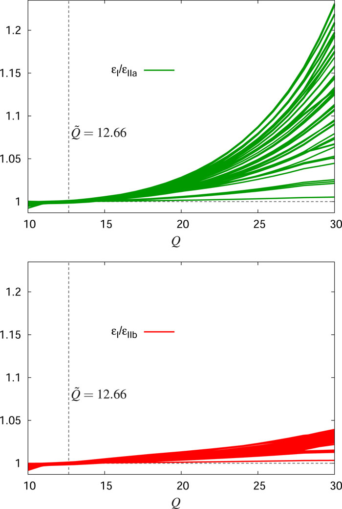
Figures 14 and 15 present comparisons of the internal energies of gold plasmas at zero radiation energy density (T_r = 0) obtained using both Eqs. (62)–(68) and (74). For Eq. (74), we employed one-electron energies and Slater integrals found both with method I [from the solution of the SCF Eqs. (30)–(39)] and method II [i.e., the NLTE one-electron energies as calculated using either Eq. (50) or Eq. (51) and isolated-ion Slater integrals for the LTE numbers of bound electrons]. The use of Eq. (74) in the context of method II enables one to rapidly evaluate thermodynamic functions, while the calculations with method I provide just a direct validity check of Eq. (74) by eliminating the effects due to minor inaccuracies in the one-electron energies and Slater integrals utilized in method II. One can see from Figs. 14 and 15 that Eq. (74) is valid at sufficiently high temperatures (T_e ≳ 0.1–1 keV), while at lower temperatures, the approximations employed to arrive at Eq. (74) lead to an essential distinction from the results obtained with the basic Eqs. (62)–(68). However, one can significantly improve the low-temperature results by taking advantage of the EOS data precalculated in the LTE approximation and using Eq. (74) just to evaluate the departure of the internal energy from the relevant LTE value rather than the total internal energy itself. In doing so, one adds the difference of NLTE and LTE energies calculated by Eq. (74) to the LTE energy given by the precalculated EOS data [generated, for example, using Eqs. (62)–(68) for the LTE case]. As one can see from Figs. 16 and 17, the adoption of this approach in the context of method I provides good agreement with the results of the SCF calculations using Eqs. (62)–(68). In the context of method II, the inaccuracy of the NLTE internal energy appears to be somewhat larger (owing to minor inaccuracies in the average ion charges and the approximate evaluation of one-electron energies and Slater integrals), although it remains much smaller than the difference between the NLTE and LTE internal energies.

Figure 14.Ratios of specific electron internal energy to free-electron temperature for gold at ρ = 10⁻² g/cm³ calculated in the LTE approximation (dashed curves) and without the use of the LTE approximation at T_r = 0 (solid curves). Blue, orange, and green curves represent the calculations using method I with Eqs. (62)–(68), method I with Eq. (74), and method IIa with Eq. (74), respectively. Two-electron processes are ignored.

Figure 16.Ratios of specific electron internal energy to free-electron temperature for gold at ρ = 10⁻² g/cm³ as calculated in the LTE approximation (cyan solid curve) and without the use of the LTE approximation at T_r = 0. The LTE energy is obtained using method I with Eqs. (62)–(68), while the departure of the NLTE energy from its LTE counterpart is evaluated using method I with the same Eqs. (62)–(68) (blue solid curve) or with Eq. (74) (orange dashed curve), or using method IIa/IIb with Eq. (74) (green solid/red dashed curve). Two-electron processes are ignored.

One can see from Figs. 18 and 19 that for the cases considered here, the pressure values obtained with the basic Eqs. (69)–(72) and the simplified Eq. (75) are fairly close. However, in the general case, it is appropriate to employ Eq. (75) just to evaluate the difference between the NLTE and LTE pressures, with the LTE pressure term being given by the precalculated EOS data. The reason is that at low temperatures and high material densities (not addressed in Figs. 18 and 19), Eq. (75) may not be accurate enough [and nor may the simplified Eq. (74) for the internal energy]. At the same time, under such conditions, the departure from LTE is generally small, and therefore the use of the simplified equation to evaluate the departure of pressure (or internal energy) from LTE values does not provide considerable errors of the total pressure (or internal energy).

Figure 18.Ratios of electron pressure to the product of the free-electron temperature and the material density for gold at ρ = 10⁻² g/cm³ as calculated in the LTE approximation (upper curves) and without the use of the LTE approximation at T_r = 0 (lower curves) using method I with Eqs. (69)–(72) (blue solid curves) and method IIa with Eq. (75) (green dashed curves). Two-electron processes are ignored.

Thus, we have proposed an efficient method to calculate the electron thermodynamic functions of NLTE plasmas involving the use of their LTE counterparts from the precalculated EOS data and the evaluation of departures from the LTE values with the simple Eqs. (74) and (75).

We have proposed and validated a simplified version of the NLTE average-atom model that employs the LTE average-atom atomic data and thermodynamic functions along with the isolated-ion atomic data. This approach facilitates fast and fairly accurate computations with no need for extensive atomic datasets and is therefore well suited for routine use in radiation-hydrodynamics codes. We have also compared average ion charges, charge state distributions, and emission spectra of gold plasmas under strong NLTE conditions obtained using collisional-radiative models employing detailed configuration accounting (THERMOS) and the representation of a single average-atom configuration supplemented by a binomial distribution of configuration probabilities and the superconfiguration approach (RESEOS). In most cases, the results of the RESEOS and more detailed THERMOS calculations are found to be in reasonable agreement both with each other and with data from benchmark measurements at the OMEGA and NOVA lasers, although in some cases we have revealed a modest underestimation of the calculated average ion charges compared with the experimental ones.

References

[1] J.Bauche, C.Bauche-Arnoult, O.Peyrusse. Atomic Properties in Hot Plasmas: From Levels to Superconfigurations(2015).
[2] A.Bar-Shalom, W. H.Goldstein, J.Oreg, D.Shvarts, A.Zigler. Super-transition arrays: A model for the spectral analysis of hot, dense plasma. Phys. Rev. A, 40, 3183-3193(1989).
[3] A.Bar-Shalom, M.Klapisch, J.Oreg. Collisional radiative model for heavy atoms in hot non-local-thermodynamical-equilibrium plasmas. Phys. Rev. E, 56, R70-R73(1997).
[4] A.Bar-Shalom, M.Klapisch, J.Oreg. Non-LTE superconfiguration collisional radiative model. J. Quant. Spectrosc. Radiat. Transfer, 58, 427-439(1997).
[5] A.Bar-Shalom, M.Klapisch, J.Oreg. Recent developments in the SCROLL model. J. Quant. Spectrosc. Radiat. Transfer, 65, 43-55(2000).
[6] O.Peyrusse. A superconfiguration model for broadband spectroscopy of non-LTE plasmas. J. Phys. B: At. Mol. Opt. Phys., 33, 4303-4321(2000).
[7] M.Busquet. Radiation-dependent ionization model for laser-created plasmas. Phys. Fluids B, 5, 4191-4206(1993).
[8] C.Bowen. NLTE emissivities via an ionisation temperature. J. Quant. Spectrosc. Radiat. Transfer, 71, 201-214(2001).
[9] C.Bowen, P.Kaiser. Dielectronic recombination in Au ionisation temperature calculations. J. Quant. Spectrosc. Radiat. Transfer, 81, 85-95(2003).
[10] M.Busquet, D.Colombant, D.Fyfe, J.Gardner, M.Klapisch. Improvements to the RADIOM non-LTE model. High Energy Density Phys., 5, 270-275(2009).
[11] R. M.More. Electronic energy levels in dense plasmas. J. Quant. Spectrosc. Radiat. Transfer, 27, 345-357(1982).
[12] P.Dallot, A.Decoster, G.Faussurier, A.Mirone. Average-ion level-population correlations in off-equilibrium plasmas. Phys. Rev. E, 57, 1017-1028(1998).
[13] E.Berthier, C.Blancard, G.Faussurier. Nonlocal thermodynamic equilibrium self-consistent average-atom model for plasma physics. Phys. Rev. E, 63, 026401(2001).
[14] C.Blancard, A.Decoster, G.Faussurier. New screening coefficients for the hydrogenic ion model including
[15] S. B.Hansen, H. A.Scott. Advances in NLTE modeling for integrated simulations. High Energy Density Phys., 6, 39-47(2010).
[16] B. F.Rozsnyai. Collisional-radiative average-atom model for hot plasmas. Phys. Rev. E, 55, 7507-7521(1997).
[17] B. F.Rozsnyai. Hot plasma opacities in the presence or absence of local thermodynamic equilibrium. High Energy Density Phys., 6, 345-355(2010).
[18] A. F.Nikiforov, V. G.Novikov, V. B.Uvarov. Quantum-statistical models of hot dense matter. Methods for Computation Opacity and Equation of State(2005).
[19] A. S.Grushin, P. A.Loboda, V. G.Novikov, A. A.Ovechkin, A. D.Solomyannaya. RESEOS—A model of thermodynamic and optical properties of hot and warm dense matter. High Energy Density Phys., 13, 20-33(2014).
[20] A. L.Falkov, P. A.Loboda, A. A.Ovechkin. Transport and dielectric properties of dense ionized matter from the average-atom RESEOS model. High Energy Density Phys., 20, 38-54(2016).
[21] D. A.Liberman. Self-consistent field model for condensed matter. Phys. Rev. B, 20, 4981-4989(1979).
[22] T.Blenski, R.Piron. Variational-average-atom-in-quantum-plasmas (VAAQP) code and virial theorem: Equation-of-state and shock-Hugoniot calculations for warm dense Al, Fe, Cu, and Pb. Phys. Rev. E, 83, 026403(2011).
[23] A.Bar-Shalom, W. H.Goldstein, J.Oreg. Effect of configuration widths on the spectra of local thermodynamic equilibrium plasmas. Phys. Rev. E, 51, 4882-4890(1995).
[24] V. G.Novikov, Y.Ralchenko. Average atom approximation in non-LTE level kinetics. Modern Methods in Collisional-Radiative Modeling of Plasmas, 105-126(2016).
[25] A. S.Grushin, D. A.Kim, A. D.Solomyannaya, I. Y.Vichev. On certain aspects of the THERMOS toolkit for modeling experiments. High Energy Density Phys., 33, 100713(2019).
[26] M. E.Foord, K. B.Fournier, D. H.Froula, S. B.Hansen, R. F.Heeter, A. J.Mackinnon, M. J.May, M. B.Schneider, B. K. F.Young. Benchmark measurements of the ionization balance of non-local thermodynamic equilibrium gold plasmas. Phys. Rev. Lett., 99, 195001(2007).
[27] J. R.Albritton, M. E.Foord, K. B.Fournier, S. H.Glenzer, P. T.Springer, R. S.Thoe, B. G.Wilson, K. L.Wong. Accurate determination of the charge state distribution in a well characterized highly ionized Au plasma. J. Quant. Spectrosc. Radiat. Transfer, 65, 231-241(2000).
[28] H.van Regemorter. Rate of collisional excitation in stellar atmospheres. Astrophys. J., 136, 906-915(1962).
[29] R. D.Cowan. The Theory of Atomic Structure and Spectra(1981).
[30] M.Blaha, H. R.Griem, P. C.Kepple. Stark-profile calculations for Lyman-series lines of one-electron ions in dense plasmas. Phys. Rev. A, 19, 2421-2432(1979).
[31] Using the relation l∼2meε/q, valid at high free-electron energies, one can rewrite the restriction q ≳ ℏ/d in a more evident form: ρ ≲ d, where ϱ≃ℏl/2meε is the classical impact parameter.
[32] W.Lotz. Electron-impact ionization cross-sections and ionization rate coefficients for atoms and ions. Astrophys. J. Suppl., 14, 207(1967).
[33] C.Blancard, G.Faussurier. Degeneracy and relativistic microreversibility relations for collisional-radiative equilibrium models. Phys. Rev. E, 95, 063201(2017).
[34] I.Sobelman. Introduction to the Theory of Atomic Spectra(1972).
[35] In the present work, we do not allow for the change of the m-subshell occupation number brought about by two-electron transitions like (j → c, m → i) and (i → c, j → m) as well as by their inverse counterparts.13 In general, the inclusion of these transitions would suggest the use of more accurate approximations to evaluate transition rates Ajimc than the dipole approximation employed in Eq. (23), e.g., the distorted-wave approximation.1 This is evidenced merely by the fact that Eq. (23) yields different values of the m → c, j → i (Ajimc) and j → c, m → i (Amijc) transition rates (so that one of these may even be equal to zero), although in the distorted-wave approximation these rates appear to be the same.
[36] In practice, the occupation numbers in Eqs. (22) and (25) are updated only when one goes from one external iteration to another, i.e., variation of those in the internal iterations is not allowed.
[37] V.Eyert. A comparative study on methods for convergence acceleration of iterative vector sequences. J. Comput. Phys., 124, 271-285(1996).
[38] B. I.Bennett, D. A.Liberman. Atomic vibrations in a self-consistent-field atom-in-jellium model of condensed matter. Phys. Rev. B, 42, 2475-2484(1990).
[39] N. M.Gill, C. W.Greeff, T.Sjostrom, C. E.Starrett. Wide ranging equation of state with tartarus: A hybrid Green’s function/orbital based average atom code. Comp. Phys. Commun., 235, 50-62(2019).
[40] R.Karazija. The Theory of X-Ray and Electronic Spectra of Free Atoms: An Introduction(1987).
[41] J.Dubau, G.Massacrier. A theoretical approach to N-electron ionic structure under dense plasma conditions: I. Blue and red shift. J. Phys. B: At. Mol. Opt. Phys., 23, 2459S-2469S(1990).
[42] M. F.Gu. The flexible atomic code. Can. J. Phys., 86, 675-689(2008).
[43] A basic configuration is built by successively filling subshells in order of increasing quantum numbers n, l, and j.
[44] X.Li, F. B.Rosmej. Quantum-number-dependent energy level shifts of ions in dense plasmas: A generalized analytical approach. Europhys. Lett., 99, 33001(2012).
[45] M.Poirier. A study of density effects in plasmas using analytical approximations for the self-consistent potential. High Energy Density Phys., 15, 12-21(2015).
[46] V. A.Astapenko, X.Li, V. S.Lisitsa, F. B.Rosmej. An analytical plasma screening potential based on the self-consistent-field ion-sphere model. Phys. Plasmas, 26, 033301(2019).
[47] C. A.Iglesias. On spectral line shifts from analytic fits to the ion-sphere model potential. High Energy Density Phys., 30, 41-44(2019).
[48] J.-C.Pain. On the Li-Rosmej analytical formula for energy level shifts in dense plasmas. High Energy Density Phys., 31, 99-100(2019).
[49] X.Li, F. B.Rosmej. Analytical approach to level delocalization and line shifts in finite temperature dense plasmas. Phys. Lett. A, 384, 126478(2020).
[50] D.Benredjem, J.-C.Pain. Simple electron-impact excitation cross-sections including plasma density effects. High Energy Density Phys., 38, 100923(2019).
[51] K. D.Pyatt, J. C.Stewart. Lowering of ionization potentials in plasmas. Astrophys. J., 144, 1203-1211(1966).
[52] In fact, THERMOS calculates atomic-process rates using the differences of average configuration energies rather than one-electron transition energies as is done in RESEOS. This distinction, however, plays no significant role in the comparisons of the RESEOS and THERMOS results presented and is therefore omitted in the following discussion.
[53] J. R.Albritton, B. G.Wilson. NLTE ionization and energy balance in high-
[54] P.Beiersdorfer, G. V.Brown, K. B.Fournier, C. L.Harris, M. J.May, P. A.Neill, P.Springer, B.Wilson, K. L.Wong. Determination of the charge state distribution of a highly ionized coronal Au plasma. Phys. Rev. Lett., 90, 235001(2003).
[55] P.Beiersdorfer, S. B.Hansen, M. J.May, J. H.Scofield. Atomic physics and ionization balance of high-Z ions: Critical ingredients for characterizing and understanding high-temperature plasmas. High Energy Density Phys., 8, 271-283(2012).
[56] F.Gilleron, J.-C.Pain. Stable method for the calculation of partition functions in the superconfiguration approach. Phys. Rev. E, 69, 056117(2004).
[57] C.Bowen, R.Florido, R. W.Lee, Y.Ralchenko, J. G.Rubiano. Review of the 4th NLTE code comparison workshop. High Energy Density Phys., 3, 225-232(2007).
[58] A. L.Falkov, P. A.Loboda, A. A.Ovechkin, P. A.Sapozhnikov. Equation of state modeling with pseudoatom molecular dynamics. Phys. Rev. E, 103, 053206(2021).
[59] O.Heuzé, J.-C.Pain, N.Wetta. D’yakov-Kontorovitch instability of shock waves in hot plasmas. Phys. Rev. E, 98, 033205(2018).
Set citation alerts for the article
Please enter your email address
© Copyright 2018-2021 | Chinese Laser Press. All Rights Reserved 沪ICP备15018463号-20