1Pohang University of Science and Technology, School of Interdisciplinary Bioscience and Bioengineering, Graduate School of Artificial Intelligence, Medical Device Innovation Center, Department of Electrical Engineering, Convergence IT Engineering, and Mechanical Engineering, Pohang, Republic of Korea
2Sungkyunkwan University, Institute of Quantum Biophysics, Department of Biophysics, Suwon, Republic of Korea
Jinge Yang, Seongwook Choi, Jiwoong Kim, Byullee Park, Chulhong Kim, "Recent advances in deep-learning-enhanced photoacoustic imaging," Adv. Photon. Nexus 2, 054001 (2023)
Copy Citation Text
Photoacoustic imaging (PAI), recognized as a promising biomedical imaging modality for preclinical and clinical studies, uniquely combines the advantages of optical and ultrasound imaging. Despite PAI’s great potential to provide valuable biological information, its wide application has been hindered by technical limitations, such as hardware restrictions or lack of the biometric information required for image reconstruction. We first analyze the limitations of PAI and categorize them by seven key challenges: limited detection, low-dosage light delivery, inaccurate quantification, limited numerical reconstruction, tissue heterogeneity, imperfect image segmentation/classification, and others. Then, because deep learning (DL) has increasingly demonstrated its ability to overcome the physical limitations of imaging modalities, we review DL studies from the past five years that address each of the seven challenges in PAI. Finally, we discuss the promise of future research directions in DL-enhanced PAI.
Photoacoustic imaging (PAI) is a noninvasive and radiation-free biomedical imaging modality that provides high spatial resolution, deep penetration, and great optical absorption contrast by synergistically combining optics and acoustics.1 PAI is based on the photoacoustic (PA) effect, in which optical energy from a pulse laser is converted into acoustic energy waves by the light absorption characteristics of biomolecules.2 The initial pressure of a generated PA wave can be calculated as where denotes the initial pressure, is the Gruneisen coefficient, is the optical absorption coefficient, is the efficiency of heat conversion from the optical absorption, and is the optical fluence. Because acoustic scattering in biological tissues is several orders of magnitude lower than light scattering, PAI can obtain biomolecule information based on the absorption contrast of light at a depth of several centimeters.3,4 PAI also extracts the concentrations of intrinsic chromophores, such as oxyhemoglobin (HbO), deoxyhemoglobin (HbR), melanin, water, and lipids, using multispectral image processing.5–13 In particular, oxygen saturation (), an important index for evaluating various diseases, is calculated through HbO and HbR values.14 By exploiting spectral characteristics, PAI can analyze physiological functions such as , blood flow, and metabolic rates in preclinical and clinical research.4,15–17 For example, the high sensitivity of PAI to hemoglobin has made it valuable in preclinical studies of angiogenic diseases, tumor hypoxia, and cerebral hemodynamics.18–20 Further, the use of PAI is expanding into clinical research areas, such as thyroid and breast cancer screening, lymph node biopsy guidance, tissue examination, and melanoma staging.21–24 Not limited to endogenous chromophores, the high molecular sensitivity of PAI enables molecular imaging when exogenous contrast agents are administered.4 Biodistribution and pharmacokinetics in the body can be imaged in vivo through exogenous contrast agents that generate PA signals.25–27 In this way, PAI is being used in diagnosing cancer and brain diseases and monitoring their therapies, in studying the organ accumulation of substances, and in tracking the dissemination of drugs.8,28–30
Photoacoustic microscopy (PAM) and photoacoustic computed tomography (PACT) are the main PAI modalities. PAM is subdivided into two types, depending on which of the two co-aligned acoustic and optical components is more tightly focused.31–36 Optical resolution PAM (OR-PAM), which implements focused optical illumination on the acoustic focal area, shows high spatial resolution (a few micrometers) and has been applied to investigate small biological structures.37,38 Acoustic resolution PAM (AR-PAM) uses a less tightly focused optical beam than OR-PAM, but its acoustic focus is smaller than its laser focus.39 AR-PAM achieves deeper light penetration (up to several centimeters, compared to the 1 mm depth in OR-PAM) despite its lower spatial resolution (tens/hundreds of micrometers), defined by the acoustic focus. PACT uses multiple detection positions to simultaneously reconstruct an image in 2D or 3D. It provides hundreds of images with micrometer-level spatial resolution at imaging depths ranging in the tens of millimeters. PACT uses a high-energy wide laser beam and an ultrasound (US) transducer array (e.g., linear, ring-shaped, arc-shaped, or hemispherical) to receive US waves generated by laser illumination.3,21,40–42 Images are created by reconstruction algorithms,43 such as delay-and-sum (DAS),44,45 delay-multiply-and-sum (DMAS),46 backprojection (BP),47 Fourier beam forming,48 time reversal (TR),49 and model-based methods.50,51
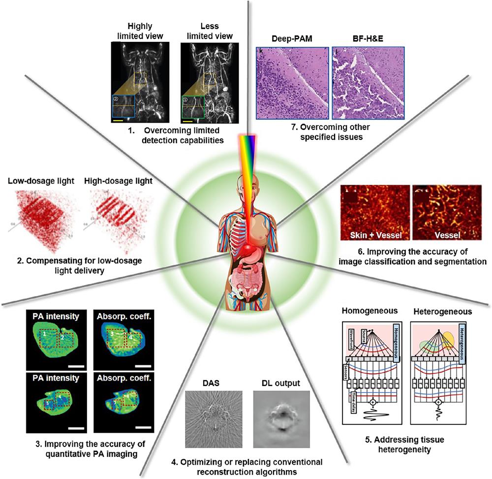
PAI has gained widespread recognition as a promising biomedical imaging modality for preclinical and clinical studies. However, to fully realize PAI’s great potential, the seven challenges listed in Table 1 and illustrated in Fig. 1 must be addressed to further enhance the image quality and expand PAI’s applications:
Sign up for Advanced Photonics Nexus TOC. Get the latest issue of Advanced Photonics Nexus delivered right to you!Sign up now
Overcoming these challenges is important because relying solely on hardware improvements will not be enough to resolve them. It will require significant investments of time and resources to find effective solutions. Deep learning (DL) plays a crucial role in advancing the field of medical and bioimaging by not only addressing the inherent limitations of imaging systems but also by driving substantial improvements in classification and segmentation performance. In recent years, DL has gained significant traction in PAI research, leading to remarkable breakthroughs and achievements. This comprehensive review article provides an in-depth analysis of diverse methodologies and outcomes showcasing the utilization of DL techniques to effectively address the seven challenges encountered in PAI, as previously outlined.
2 Principles of DL Methods
DL is a subset of machine-learning algorithms that encompasses supervised learning, unsupervised learning, and reinforcement learning. Supervised learning is a modeling technique that establishes a correlation between input data and their corresponding ground truth (GT). This approach is commonly utilized in DL-enhanced medical imaging, where high- and low-quality images can be paired. On the other hand, unsupervised learning identifies specific patterns hidden within data, without the use of labeled examples or a priori known answers. Lastly, in reinforcement learning, an algorithm maximizes the final reward by learning through rewards obtained as a result of performing specific actions in a particular environment. A notable example of such a learning algorithm is AlphaGo, the first computer program to beat a human champion Go player.63 Next, we explain the basic structure of DL network and the basic operating principle of DL training. In addition, we introduce the representative DL architectures that are most widely used in the field of image and video: convolution neural network (CNN), U-shaped neural network (U-Net), and generative adversarial network (GAN) architecture.
2.1 Artificial Neural Networks
Artificial neural networks (ANNs) draw inspiration from biological neural networks, wherein different stimuli enter neurons through dendrites and are transmitted to other cells through axons once a threshold of activation is achieved [Fig. 2(a)]. In ANNs, an artificial neuron is a mathematical function conceived as a biological neuron. This function multiplies the various inputs by each weight, sums them, and adds the deviation.
Figure 2.The concept of (a) a biological neural network and (b) an ANN derived from (a). (c) Schematics of a simple neural network and a DNN.
This sum is then sent to a specific activation function and produces an output [Fig. 2(b)]. This artificial neuron is expressed as where is the activation function, is the input, is the weight, is the variance, and is the output. The calculated output acquires nonlinearity through such activation functions () as sigmoid, hyperbolic tangent, and rectified linear unit.64 Without such an activation function, it would be pointless to build a deep model, since a linear transformation would occur regardless of how many hidden layers are present.
ANNs typically have an input layer, a hidden layer, and an output layer, each comprising multiple units. The number of hidden layers between the input and output determines whether the ANN is a simple neural network or a deep neural network (DNN) [Fig. 2(c)]. Formulaically, the two networks in Fig. 2(c) are described as and
2.2 Backpropagation
Backpropagation serves as the fundamental principle for training DL models. In order to grasp the concept of backpropagation, it is necessary to first understand forward propagation. Forward propagation involves sequentially passing an input value through multiple hidden layers to generate an output. For instance, given an input , a weight , a variance , and an activation function , the DNNs’ forward propagation on Fig. 2(c) is represented as where represents the value predicted by DNNs. The process of finding the optimized and variables that minimize the loss, which is the difference between the predicted result and the actual , is called training. The loss is calculated for all training data sets. As loss-function metrics, image data sets such as PA images commonly employ the structural similarity index measure (SSIM) and peak-signal-to-noise ratio (PSNR). Backpropagation refers to the process of transmitting the loss back to the input stage using the chain rule.65,66 This process determines the weight that yields the minimal loss function value. Most DL models adopt the gradient descent technique throughout this procedure.67 By calculating the gradient at a specific and continually updating , the loss function’s minima can be estimated using the following equation:
The learning rate, a hyperparameter that determines the variable’s update amount in proportion to the calculated slope, is set before the learning process and remains unchanged. The number of hidden layers and their dimensions are also hyperparameters. In the following section, we introduce representative ANN architectures commonly used in biomedical imaging, including PAI.
2.3 CNN
CNNs, the most basic DL architecture, have received significant attention in the field of PAI due to their extensive use in image processing and computer vision. CNNs were developed to extract features or patterns in local areas of an image. A convolution operation is a mathematical process that measures the similarity between two functions. The convolution operation in image processing is the process of calculating how well a subsection of an image matches a filter (also referred to as a kernel) and is used for things such as edge filtering. In CNN, the network is trained by learning this filter, which is used to extract image features, as a weight. The encoder–decoder CNN architecture is a relatively simple network structure capable of performing image-to-image translation tasks [Fig. 3(a)].68 Initially, the input image undergoes a series of downsampling and convolution operations. Throughout this process, the dimensions of the image progressively decrease while the number of image channels, representing an additional dimension, increases. This results in a bottleneck in the representation, which is subsequently reversed through a sequence of upsampling and convolutional operations. The bottleneck enforces the network to encode the image into a compact set of abstracted variables (also referred to as latent variables) along the channel dimension. The predicted image is synthesized by decoding these variables in the second half of the network.
Figure 3.Three typical neural network architectures for biomedical imaging. (a) CNN, (b) U-Net, and (c) GAN.
A U-Net [Fig. 3(b)] is a CNN-based model that was originally proposed for image segmentation in the biomedical field.69 The U-Net is composed of two symmetric networks: a network for obtaining overall context information of an image and a second network for accurate localization. The left part of the U-Net is the encoding process, which encodes the input image to obtain overall context information. The right part of U-Net is the decoding process, which decodes the encoded context information to generate a segmented image. The feature maps obtained during the encoding process are concatenated with up-convolved feature maps at each expanding step in the decoding process, using skip connections.70 This enables the decoder to make more accurate predictions by directly conveying important information in the image. As a result, the U-Net architecture has shown excellent performance in several biomedical image segmentation tasks, even when trained on a very small amount of data, due to data augmentation techniques.
2.5 GAN
A GAN is a type of generative model that learns data through a competition between a generator network and a discriminator network [Fig. 3(c)].71,72 The generator network generates the fake data, and the discriminator network tries to distinguish the real data from the fake data. To deceive the discriminator, the generator aims to generate data that look as realistic as possible, while the discriminator attempts to distinguish the real data from the realistic fake data. Through this competition, both networks learn and improve iteratively, resulting in a generator that can generate increasingly realistic data. As a result, GANs have been successful in generating synthetic data that are very similar to real data, making them useful for applications such as data augmentation and image synthesis. These three representative networks are summarized in Table 2.
Network
Key feature
Use case
CNN
Performs convolution operation for feature extraction.
Image enhancement
Exhibits outstanding performance in feature extraction.
Image classification and object detection
Captures spatial information of input data efficiently.
Image segmentation
U-Net
Comprises an encoder–decoder structure.
Image enhancement
Utilizes skip connections to leverage high-resolution feature maps.
Demonstrates strong performance even with small data sets.
Image segmentation
Excels in segmentation tasks.
GAN
Consists of a generator network and a discriminator network.
Image generation
Generates data that closely resembles real input data (generator).
Discriminates between generated data and real data (discriminator).
Image style transfer
Engages in competitive training between the generator and discriminator.
In PAI, optimal image quality requires a broadband US transducer and dense spatial sampling to enclose the target.43,61,73 However, real-world scenarios introduce limitations, such as limited bandwidth, limited view, and data sparsity. DL methods have been used as postprocessing techniques to overcome these limitations and enhance the PA signals or images, reducing artifacts. This section provides an overview of studies utilizing DL methods as PAI postprocessing methods. The DL-based image reconstruction studies are discussed separately in Sec. 3.4.
3.1.1 Limited bandwidth
The bandwidth of US transducer arrays is limited compared to the natural broadband PA signal (from tens of kilohertz to a hundred megahertz).74 Although optical detectors of PA waves have expanded the detection bandwidth, manufacturing high-density optical detector arrays and adopting them to PACT remains a technical challenge.75
To solve the limited-bandwidth problem, Gutte et al. proposed a DNN with five fully connected layers to enhance the PA bandwidth [Fig. 4(a)].76 The network takes a limited-bandwidth signal as input and outputs an enhanced bandwidth signal, which is then used for PA image reconstruction using DAS. To train the network, the authors generated numerical phantoms using the k-Wave toolbox79 to create pairs of full-bandwidth and limited-bandwidth PA signals. The synthesized results from the numerical phantoms demonstrated an enhanced bandwidth that is like that of images obtained from the full-bandwidth signal [Fig. 4(a)].
PA image quality is reduced by the scant information provided by the limited coverage angle of the PA signals detected by the US transducer.3 This problem is commonly encountered in PACT systems, particularly in linear US array-based systems and is referred to as the “limited view” problem.75,80 Researchers have addressed this problem to some extent by developing reconstruction methods with iterative methods.80 Recent studies based on the fluctuation of the PA signal of blood flow or microbubbles81,82 show another effective solution, but they need a number of single images to reconstruct one fluctuation image, which compromises the temporal resolution.
Deng et al.83 developed DL methods using U-Net and principal component analysis processed very deep convolutional networks (PCA-VGG)84 while Zhang et al.85 designed a dual domain U-Net (DuDoUnet) incorporating reconstructed images and frequency domain information. In addition to utilizing the U-Net architecture, researchers have also explored the use of GAN networks, which have garnered attention due to their ability to preserve high-frequency features and prevent oversmoothing in images. Lu et al. proposed a GAN-based network called the limited view GAN (LV-GAN).77Figure 4(b) shows the architecture of LV-GAN, which consists of two networks: the generator network responsible for generating high-quality PA images from limited-view images, and the discriminator network designed to distinguish the generated images from the GT. To ensure accurate and generalizable results, the LV-GAN was trained using both simulated data generated by the k-Wave toolbox and experimental data obtained from a custom-made PA system. The results presented in Fig. 4(b), using ex vivo data, demonstrate the ability of LV-GAN to successfully reconstruct high-quality PA images in limited-view scenarios. The quantitative analysis further confirms that LV-GAN outperforms the U-Net framework, achieving the highest retrieval accuracy.
The combination of a postprocessing method with direct processing using PA signals is considered as another approach to reduce artifacts in limited-view scenarios. Lan et al.78 designed a new network architecture, called Y-net, which reconstructs PA images by optimizing both raw data and reconstructed images from the traditional method [Fig. 4(c)]. This network has two inputs, one from raw PA data and the other from the traditional reconstruction. It combines two encoders, each corresponding to one of the input paths, with a shared decoder path. The training data were generated by the k-Wave toolbox with a linear array setup. The public vascular data set86 was used to generate PA signals. They compared the proposed method with conventional reconstruction methods [e.g., DAS and time reversal (TR)] and other DL methods such as U-Net. In in vitro and in vivo experiments, the proposed method showed superior performance to the other methods, with the best spatial resolution.
3.1.3 Sparsity
To achieve the best image quality, the interval between two adjacent positions of the transducer or array elements must be less than half of the lowest detectable acoustic wavelength, according to the Nyquist sampling criterion.87 In sparse sampling, the actual detector density is lower than this requirement, introducing streak-shaped artifacts in images.74 Sparse sampling can also result from a trade-off between image quality and temporal resolution, which is sometimes driven by system cost and hardware limitations.88
To remove artifacts caused by data sparsity, Guan et al.89 added additional dense connectivity into the contracting and expanding paths of a U-Net. Farnia et al.90 combined a TR method with a U-Net by inserting it in the first layer. Guo et al.91 built a network containing a signal-processing method and an attention-steered network (AS-Net). Lan et al.92 proposed a knowledge infusion GAN (Ki-GAN) architecture that combines DAS and PA signals for reconstruction from sparsely sampled data. DiSpirito et al.93 compared various CNN architectures for PAM image recovery from undersampled data of in vivo mouse brains.94 They chose a fully dense U-Net (FD U-Net) with a dense block, allowing PAM image reconstruction using just 2% of the original pixels. Later, they proposed a new method based on a deep image prior (DIP) method95 to solve this problem without pretraining or GT data.
3.1.4 Combinational limited-detection problems
Previous studies have primarily tackled individual issues in isolation, neglecting the simultaneous occurrence of multiple limited-detection challenges in PA systems.74 However, researchers have recently focused on utilizing a single NN to address two or three limited-detection problems concurrently, leading to promising advancements in this area.
For linear array, Godefroy et al.96 incorporated dropout layers97 into a modified U-Net and further built a Bayesian NN to improve the PA image quality. Vu et al.98 built a Wasserstein GAN (WGAN-GP) that combined a U-Net and a deep convolutional GAN (DCGAN).99 The network reduced limited-view and limited-bandwidth artifacts in PACT images. For a ring-shaped array, Zhang et al.100 developed a 10-layer CNN, termed a ring-array DL network (RADL-net), to eliminate limited-view and under-sampling artifacts in photoacoustic tomography (PAT, also known as PACT) images. Davoudi et al.101 proposed a U-Net network to improve the image quality from sparsely sampled data from a full-ring transducer array. They later updated their U-Net architecture102 to operate on both images and PA signals. Awasthi et al.103 proposed a U-Net architecture to achieve superresolution, denoising, and bandwidth enhancements. They replaced the softmax activation function in the final two layers of the U-Net for segmentation with an exponential linear unit.104 Schwab et al. proposed a network that combined the BP with dynamic aperture length (DAL) correction, which they called DALnet105 to address the limited-view and undersampling issues in the 3D imaging PACT system.
One of the notable achievements in applying DL to the 3D-PACT system was made by Choi et al.52 They introduced a 3D progressive U-Net (3D-pUnet) as a solution to address limited-view artifacts and sparsity caused by clustered-sampling detection, as shown in Fig. 4(d). The design of their network was inspired by the progressive growth GAN,106 which utilizes a progressively increasing procedure to optimize a U-Net. In their 3D-pUnet, subnetworks were trained sequentially using downsampled data from the original high-resolution volume data, gradually transferring knowledge obtained from each progressive step.
The training data set consisted of in vivo experimental data from rats, and the results demonstrated superior performance compared with the conventional 3D-U-Net method. Interestingly, they demonstrated that the 3D-pUnet trained cluster-sampled data set also works in sparsely sampled data sets. The proposed approach was also applied to predict dynamic contrast-enhanced images and functional neuroimaging in rats, achieving increased imaging speed while preserving high image quality. In addition, they demonstrated the ability to accurately measure physiological phenomena and enhance structural information in untrained subjects, including tumor-bearing mice and humans.
All the research reviewed in this section is summarized in Table 3.
Author
Neural network architecture
Basic network
Training data set (if specified, validation is excluded)
Test data set
Specified task
Representative evaluation results
Source
Data amount
Gutte et al.76
FC-DNN
CNN
Simulation of the breast phantom
286,300 slices (from 2863 volumes)
Simulation/in vitro phantom
Reduce limited-bandwidth artifacts
CNR (versus DAS) 0.01 → 2.54
PC 0.22 → 0.75
Deng et al.83
U-Net and VGG
U-Net
In vivo mouse liver
50
Numerical simulation data/in vitro phantom/in vivo data
Reduce limited-view artifacts from the circular US array
SSIM (versus DAS) 0.39 → 0.91
PSNR 7.54 → 24.34
Zhang et al.85
DuDoUnet
U-Net
k-Wave simulation
1500
k-Wave simulation
Reduce limited-view artifacts from the linear US array
SSIM (versus U-Net) 0.909 → 0.935
PSNR 19.4 → 20.8
Lu et al.77
LV-GAN
GAN
k-Wave simulation of absorbers and vessels/in vitro phantom of microsphere and vessel structure
793 pairs (absorbers)/1600 pairs (vessels)/
k-Wave simulation of absorbers and vessels/in vitro phantom (microsphere and vessel structure)
Reduce limited-view artifacts from the circular US array
SSIM (versus DAS) 0.135 → 0.871
30 pairs (microsphere)
PSNR 9.41 → 30.38
CNR 22.72 → 43.41
22 pairs (vessel structures)
Lan et al.78
Y-Net
—
k-Wave simulation of segmented blood vessels from DRIVE data set
4700
k-Wave simulation/in vitro phantom/in vivo human palm
Reduce limited-view artifacts from the linear US array
SSIM (versus DAS) 0.203 → 0.911
PSNR 17.36 → 25.54
SNR 1.74 → 9.92
Guan et al.89
FD-UNet
U-Net
k-Wave simulation:/k-Wave simulation of realistic vasculature phantom from micro-CT images of mouse brain
1000 simulation/1000 (realistic vasculature)
k-Wave simulation:/k-Wave simulation of realistic vasculature phantom (micro-CT images of the mouse brain)
Reduce artifacts from sparse data in the circular US array
SSIM (versus DAS) 0.75 → 0.87
PSNR 32.48 → 44.84
Farnia et al.90
U-Net
U-Net
k-Wave simulation from the DRIVE data set
3200
k-Wave simulation from DRIVE data set/in vivo mouse brain
Reduce artifacts from sparse data in the circular US array
SSIM (versus DAS) 0.81 → 0.97
PSNR 29.1 → 35.3
SNR 11.8 → 14.6
EPI 0.68 → 0.90
Guo et al.91
AS-Net
Non
k-Wave simulation of human fundus culi vessel/in vivo fish/in vivo mouse
3600/1744/1046
k-Wave simulation of human fundus culi vessel/in vivo fish/in vivo mouse
Reduce artifacts from sparse data and speed up reconstruction from the circular US array
SSIM (versus DAS) 0.113 → 0.985
PSNR 8.64 → 19.52
Lan et al.92
Ki-GAN
GAN
k-Wave simulation of retinal vessels from public data set
4300
k-Wave simulation of retinal vessels from public data set
Remove artifacts from sparse data from the circular US array
SSIM (versus DAS) 0.215 → 0.928
PSNR 15.61 → 25.51
SNR 1.63 → 11.52
DiSpirito et al.93
FD U-Net
U-Net
In vivo mouse brain
304
In vivo mouse brain
Improve the image quality of undersampled PAM images
SSIM (versus zero fill) 0.510 → 0.961
PSNR 16.94 → 34.04
MS-SSIM 0.585 → 0.990
MAE 0.0701 → 0.0084
MSE 0.0027 → 0.00044
Vu et al.95
DIP
CNN
In vivo blood vessels
—
In vivo blood vessels/non-vascular data
Improve the image quality of undersampled PAM images
SSIM (versus bilinear) 0.851 → 0.928
PSNR 25.6 → 31.0
Godefroy et al.96
U-Net/Bayesian NN
U-Net
Pairs of PAI and photographs of leaves/Corresponded numerical simulation
500
PAI and photographs of leaves/numerical simulation
Reduce limited-view and limited-bandwidth artifacts from the linear US array
NCC (versus DAS) 0.31 → 0.89
SSIM 0.29 → 0.87
Vu et al.98
WGAN-GP
GAN
k-Wave simulation: disk phantom and TPM vascular data
4000 (disk)/7200 (vascular)
k-Wave simulation: disk phantom and TPM vascular data/tube phantom/in vivo mouse skin
Reduce limited-view and limited-bandwidth artifacts from the linear US array
SSIM (versus U-Net) 0.62 → 0.65
PSNR 25.7 → 26.5
Zhang et al.100
RADL-net
CNN
k-Wave simulation
161,000 (including augmentation and cropping from 126 vascular images)
k-Wave simulation/vascular structure phantom/in vivo mouse brain
Reduce limited-view and sparsity artifacts from the ring-shaped US array
SSIM (versus DAS) 0.11 → 0.93
PSNR 17.5 → 23.3
Davoudi et al.101
U-Net
U-Net
Simulation: planar parabolic absorber and mouse/in vitro circular phantom/in vitro vessel-structure phantom/in vivo mouse
Not mentioned/28/33/420
Simulation: planar parabolic absorber and mouse/in vitro circular phantom/in vitro vessel-structure phantom/in vivo mouse
Reduce limited-view and sparsity artifacts from the circular US array
SSIM (versus input) 0.281 → 0.845
Davoudi et al.102
U-Net
U-Net
In vivo human finger from seven healthy volunteers
4109 (including validation)
In vivo human finger
Reduce the limited-view and sparsity artifacts from the US circular array
SSIM (versus U-Net) 0.845 → 0.944
PSNR 14.3 → 19.0
MSE 0.04 → 0.014
NRMSE 0.818 → 0.355
Awasthi et al.103
Hybrid end-to-end U-Net
U-Net
k-Wave simulation from breast sinogram images
1000
k-Wave simulation of the numerical phantom, blood vessel, and breast/ horsehair phantoms/ in vivo rat brain
Super-resolution, denoising, and bandwidth enhancement of the PA signal from the circular US array
PC (versus DAS) 0.307 → 0.730
SSIM 0.272 → 0.703
RMSE 0.107 → 0.0617
Schwab et al.105
DALnet
CNN
Numerical simulation of 200 projection images from 3D lung blood vessel data
3000 (after cropping)
Numerical simulation/in vivo human finger
Reduce limited-view, sparsity and limited bandwidth artifacts
SSIM (versus input) 0.305 → 0.726
Correlation 0.382 → 0.933
Choi et al.52
3D-pUnet
U-Net
In vivo rat
1089
In vivo rat/in vivo mouse/in vivo human
Reduce limited-view and sparsity artifacts
MS-SSIM (versus input) 0.83 → 0.94
PSNR 32.0 → 34.8
RMSE 0.025 → 0.019
Table 3. Summary of overcoming the limited detection capabilities with DL approaches.
Pulsed laser sources, such as an optical parametric oscillator laser system with a Nd:YAG pumped laser, are commonly used in PACT systems to achieve deep penetration with a high SNR, but those laser systems are bulky and expensive.2,107 In recent years, researchers have explored compact and less expensive alternatives, such as pulsed-laser diodes107 and light-emitting diodes (LEDs).108 While these alternatives have shown promising results, their low pulse energy results in a low SNR, requiring frame averaging to increase image quality. Unfortunately, this method comes at a cost, as it reduces imaging speed. Furthermore, in dynamic imaging, frame averaging can cause blurring or ghosting due to the movement of the object being imaged. To address these problems, DL methods can be applied to enhance image quality in situations where the light intensity is low.
One of the representative works for LED-based systems was achieved by Hariri et al.53 They proposed a multilevel wavelet-convolutional NN (MWCNN) that could map the low-fluence PA images to high-fluence PA images from an Nd:YAG laser system. This approach helps to eliminate the background noise while preserving the structures of the target, as shown in Fig. 5(a). Phantom and in vivo studies were conducted to assess the performance of their model. The MWCNN demonstrated a significant improvement in contrast-to-noise ratio (CNR) with up to a 4.3-fold enhancement in the phantom study and a 1.76-fold enhancement in the in vivo study. These results highlight the practicality of the proposed method in real-world scenarios. Singh et al.111 and Anas et al.112 proposed a U-Net and a deep CNN-based approach to improve the image quality with a similar system setup. Anas et al. later introduced a recurrent neural network (RNN)113 to further improve the system’s performance.114
To enhance the image quality in a pulsed-laser-diode PA system, Rajendran et al.109 proposed a hybrid dense U-Net (HD-UNet) [Fig. 5(b)]. To train the network, they generated simulated data using the k-Wave toolbox, and evaluated the model with both single- and multi-US transducer (1-UST and multi-UST-PLD) PACT systems, using both phantom and in vivo images. Compared with their previous system, the HD-UNet improved the imaging speed by approximately 6 times in the 1-UST system and 2 times in the multi-UST-PLD system. To address the challenges of balancing laser dosage, imaging speed, and image quality in OR-PAM, Zhao et al.110 proposed a multitask residual dense network (MT-RDN) that performs image denoising, superresolution, and vascular enhancement [Fig. 5(c)]. The network comprises three subnetworks, each using an independent RDN framework and assigned a supervised learning task. The first subnetwork processes the data of input 1 (i.e., 532 nm data) to obtain output 1, and the second subnetwork processes the data of input 2 (i.e., 560 nm data) to obtain output 2. These outputs are then combined and processed by subnetwork 3, and the differences between the outputs and the GT are compared.
To train the network, input images were undersampled at half-per-pulse laser energy of the GT, while the GT images were sampled at the full ANSI per-pulse fluence limit. To evaluate the performance of the proposed method, U-Net and RDN were used. The MT-RDN method achieved a 16-fold reduction in laser dosage at 2 times data undersampling and a 32-fold reduction in dosage at 4 times undersampling compared to the GT images.
All the research reviewed in this section is summarized in Table 4.
Author
Neural network architecture
Basic network
Training data set (if specified, validation is excluded)
Test data set
Specified task
Representative evaluation results
Source
Data amount
Hariri et al.53
MWCNN
U-Net
Agarose hydrogel phantom: LED-based PA image and Nd:YAG-based PA image
229
Agarose hydrogel phantom of LED-based PA image/in vivo mouse
Denoise PA images from low-dosage system
SSIM (versus input) 0.63 → 0.93
PSNR 15.58 → 53.88
Singh et al.111
U-Net
U-Net
LED-based and Nd:YAG-based tube phantom
150
LED-based phantom using ICG and MB
Reduce the frame averaging
SNR 14 → 20
Anas et al.112
—
CNN
In vitro phantom
4536
In vivo fingers
Improve the quality of PA images
SSIM (versus average) 0.654 → 0.885
PSNR 28.3 → 36.0
Anas et al.114
—
CNN and LSTM
In vitro wire phantom/in vitro nanoparticle phantom
352,000
In vitro phantom/in vivo human fingers
Improve the quality of PA images
SSIM (versus input) 0.86→0.96
PSNR 32.3 → 37.8
Rajendran et al.109
HD-Unet
U-Net
k-Wave simulation
450
In vitro phantom/in vivo rat
Improve the frame rate
SSIM (versus U-Net) 0.92 → 0.98
PSNR 28.6 → 32.9
MAE 0.025 → 0.017
Zhao et al.110
MT-RDN
—
In vivo mouse brain and ear
6696
In vivo mouse brain and ear
Improve the quality from low dosage laser and downsampled data
SSIM (versus input) 0.64 → 0.79
PSNR 21.9 → 25.6
Table 4. Summary of studies on compensating for low-dosage light delivery.
Quantitative photoacoustic imaging (qPAI) quantifies molecular concentrations in biological tissue using multiwavelength PA images, enabling the estimation of various endogenous and exogenous contrast agents and physiological parameters, such as .61 However, qPAI presents significant challenges due to the wavelength-dependent nature of light absorption and scattering, leading to varying levels of light attenuation across different wavelengths.2,115 Thus, it is hard to accurately determine the fluence distribution, which is nonlinear and complex in biological tissues. Early research in qPAI assumed constant optical properties of biological tissue and uniform parameters such as the scattering coefficient throughout the imaging field.61 However, recent studies have shown that these assumptions lead to errors, especially in deep-tissue imaging.116 Model-based iterative optimization methods have been developed to address this issue and provide more accurate solutions.117 But these methods are time-consuming and sensitive to quantification errors.118 A new approach called eigenspectral multispectral optoacoustic tomography (eMSOT) has been proposed to improve qPAI accuracy.116 eMSOT formulates light fluence in tissues as an affine function of reference base spectra, leading to improved accuracy in qPAI. However, it requires ad hoc inversion and has limitations in scale invariance.
Researchers have pursued multiple avenues to extract fluence distribution information from multiwavelength PA images using DL architectures. Cai et al.119 introduced ResU-Net, which adds a residual learning mechanism to the U-Net. Chang et al.120 developed DR2U-Net, a fine-tuned deep residual recurrent U-Net. Luke et al.121 combined two U-Nets to create a new network called O-Net, which segments blood vessels and estimates . A novel DL architecture that contains an encoder, decoder, and aggregator was introduced by Yang et al.122 termed called EDA-Net. The encoder and decoder paths both feature a dense block, while the aggregator path incorporates an aggregation block. Gröhl et al.123 designed a nine-layer fully connected NN that directly estimates from PA images. All showed much high accuracy in estimating distributions or other molecular concentrations compared with linear unmixing.
One of the representative results is from Ref. 124. Researchers built two separated convolutional encoder–decoder type networks with skip connections, termed EDS to solve this problem in 3D conditions [Fig. 6(a)]. One network was trained to output images of from 3D-image data and the other network was trained to segment vessels. By leveraging the spatial information present in the 3D images, the 3D fully convolutional networks could produce precise maps. Besides getting more accurate results, these networks were able to handle limited-detection capabilities, such as limited-view artifacts, and showed promise for producing accurate estimates in vivo.
Researchers have also employed DL methods to recover the absorption coefficient from reconstructed PA images. Chen et al.126 proposed a U-Net-based DL network to recover the optical absorption coefficient and Grohl et al.127 adapted a U-Net to compute error estimates for optical parameter estimations. A notable contribution was made by Li et al. in a recent study.54 They addressed the challenge of insufficient data-label pairs in qPAI by introducing two DNNs, depicted in Fig. 6(b). First, they introduced a simulation-to-experiment end-to-end data translation network (SEED-Net) that provides GT images for experimental images through unsupervised data translation from a simulation data set. They then designed a dual-path network based on U-Net (QPAT-Net) to reconstruct images of the absorption coefficient for deep tissues. The QPAT-Net outperformed the previous QPAT method128 in simulation, ex vivo, and in vivo, with more accurate absorption information and relatively few errors.
Another seminal study was done by Zou et al.125 They developed the US-enhanced U-Net model (US-Unet), which combines information from US images and PA images to reconstruct the optical absorption distribution [Fig. 6(c)]. They implemented a pretrained ResNet-18 to extract features from US images of ovarian lesions.
This feature information was incorporated into a U-Net structure designed to reconstruct the optical absorption coefficient. The U-Net was trained on simulation data and subsequently tested on a phantom, blood tubes, and clinical data from 35 patients. The US-Unet outperformed both the U-Net model without US features and the standard DAS method in phantom and clinical studies, demonstrating its potential for improving accuracy in clinical PAI applications.
Compensating for the distribution of light fluence can improve the accuracy of qPAI.129–131 To this end, Madasamy et al.132 compared the compensation performance of different DL models. The models tested included U-Net,69 FD U-Net,89 Y-Net, FD Y-Net,78 deep residual U-Net (deep ResU-Net),133 and GAN.134 Results showed the robustness of all DL models to noise and their effectiveness; FD U-Net showed the best performance. qPAI requires an unmixing process, which can be achieved through linear or model-based methods.115 Durairaj et al.135 proposed an unsupervised learning approach using an initialization network and an unmixing network. Olefir et al.136 introduced DL-eMSOT, combining eMSOT with a bidirectional RNN and CNN blocks for accurate estimation and faster calculations.
All the research reviewed in this section is summarized in Table 5.
Author
Neural network architecture
Basic network
Training data set (if specified, validation is excluded)
Test data set
Specified task
Representative evaluation results
Source
Data amount
Cai et al.119
ResU-net
U-Net
Numerical simulation
2048
Numerical simulation
Extract information from multispectral PA images
Relative errors (versus linear unmixing) 36.9% → 0.76%
Chang. et al.120
DR2U-net
U-Net
Monte Carlo simulation of simulated tissue structure
2560
Monte Carlo simulation of simulated tissue structure
Extract fluence distribution from optical absorption images
Relative Errors (versus linear unmixing) 48.76% → 1.27%
Luke et al.121
O-Net:
U-Net
Monte Carlo simulation of epidermis, dermis, and breast tissue
1600 pairs (one pair has two-wavelength PA data)
Monte Carlo simulation of epidermis, dermis, and breast tissue
Estimate the oxygen saturation and segment
Relative errors (versus linear unmixing) 43.7% → 5.15%
Yang et al.122
EDA-net
—
Monte Carlo and k-Wave simulation from female breast phantom
4888
Monte Carlo and k-Wave simulation based on clinically obtained female breast phantom
Extract the information from the multi-wavelength PA images
Relative errors (versus linear unmixing) 41.32% → 4.78%
Gröhl et al.123
Nine-layer fully connected NN
CNN
Monte Carlo simulation of in silico vessel phantoms
776
In vivo porcine brain and human forearm
Obtain quantitative estimates for blood oxygenation
No statistical results
Bench et al.124
EDS
U-Net
k-Wave simulation of human lung from lung CT scans/k-Wave simulation of three-layer skin model
—
k-Wave simulation
Produce 3D maps of vascular and vessel positions
Mean difference (versus linear unmixing) 6.6% → 0.3%
Chen et al.126
U-Net
U-Net
Monte Carlo simulation
2880
In vitro phantom
Recover the optical absorption coefficient
Relative error less than 10%
Gröhl et.al127
U-Net
U-Net
Monte Carlo and k-Wave simulations of in silico tissue
3600
Monte Carlo and k-Wave simulation of in silico
Improve optical absorption coefficient estimation
Estimation error (versus linear unmixing) 58.3% → 3.1%
Li et al.54
Two GANs: SEED-Net and QOAT-Net
GAN
Numerical simulation of phantom, mouse, and human brain/experimental data of phantom, ex vivo, and in vivo mouse
3040, 2560, and 2560/2916, 3200, and 3800
Ex vivo porcine tissue, mouse liver, and kidney/In vivo mouse
Improve optical absorption coefficient estimation
Relative errors (versus linear unmixing) 8.00% → 4.82%
Relative errors 8.00% → 4.82%
Zou et al.125
US-Unet
U-Net
Monte Carlo and k-Wave simulation/in vitro phantom
2000/480
In vitro blood tube/in vivo clinical data set
Improve optical absorption coefficient estimation
Accuracy (versus linear unmixing) 0.71 → 0.89
Madasamy et al.132
Network comparing: U-Net, FD U-Net, Y-Net, FD Y-Net, Deep ResU-Net, and GAN
—
2D numerical simulation of retinal fundus (from Kaggle and RFMID)/3D numerical simulation of breast phantom
1858 (before augmentation)/5 3D volumes (12,288 slices after augmentation)
2D numerical blood vessel/3D numerical breast phantom
Fluence correction
PSNR (versus linear unmixing) 37.9 → 45.8
SSIM 0.80 → 0.96
Durairaj et al.135
Two networks: initialization network and unmixing network
—
NIRFAST and k-Wave simulation
Not mentioned
NIRFAST and k-Wave simulation
Unmix the spectral information
Regardless of prior spectral information
Olefir et al.136
DL-eMSOT: bi-directional RNN with two LSTMs
—
Monte Carlo simulation
10,944
In vitro phantom/in vivo mouse
Replace inverse problem of eMSOT
Mean error (versus eMSOT) 4.9% → 1.4%
Median error 3.5% → 0.9%
Standard deviation 4.8% → 1.5%
Table 5. Summary of studies to improve the accuracy of quantitative PAI.
3.4 Optimizing or Replacing Conventional Reconstruction Algorithms
In PACT, the acoustic inverse problem involves reconstructing the PA initial pressure from raw data. Several reconstruction methods have been developed, including BP,47 FB,48 DAS,44 DMAS,46 TR,49 and model-based methods.51 However, each method has limitations, and either to enhance existing reconstruction techniques or to directly reconstruct PA images using NNs, researchers have turned to DL methods.
Various DL methods have been developed to convert PA raw data into images. One such method, called Pixel-DL, proposed by Guan et al.,137 uses pixel-wise interpolation followed by an FD U-Net for limited-view and sparse PAT image reconstruction [Fig. 7(a)]. The Pixel-DL model was trained and tested using simulated PA data from synthetic, mouse brain, lung, and fundus vasculature phantoms. It achieved comparable or better performance than iterative methods and consistently outperformed other CNN-based approaches for correcting artifacts.
To direct reconstruct PA images, Waibel et al.139 introduced a modified U-Net that includes additional convolutional layers in each skip connection. Antholzer et al.140 proposed a direct reconstruction process, based on a U-Net and a simple CNN, that can resolve limited-view and sparse-sampling issues. Lan et al.141 proposed a modified U-Net, termed DU-Net, to reconstruct PA images using multifrequency US-sensor raw data. A noteworthy study of this topic is an end-to-end reconstruction network developed by Feng et al.,138 termed Res-U-Net [Fig. 7(b)]. They integrated residual blocks into the contracting and symmetrically expanding path of U-Net and added a skip connection between the input of raw data and the output of images. The training, validation, and test data sets were synthesized using the k-Wave toolbox. In digital phantom experiments, the Res-UNet showed performance superior to other reconstruction methods [Fig. 7(b)].
Another representative work was done by Tong et al.55 They proposed a novel two-step reconstruction process with a feature projection network (FPnet) and a U-Net [Fig. 7(c)]. The FPnet converts PA signals to images and contains several convolutional layers to extract features. There is one max pooling layer for downsampling and one full connection layer for domain transformation. The U-Net performs postprocessing to improve image quality. The resulting network, trained using numerical simulations and in vivo experimental data, outperformed other approaches to handle limited-view and sparsely sampled experimental data, exhibiting superior performance on in vivo experiments [Fig. 7(c)].
In addition, Yang et al.142 introduced recurrent inference machines (RIM), an iterative PAT reconstruction method using convolution layers. Kim et al.143 employed upgUNET, a U-Net model with 3D transformed arrays for image reconstruction. Hauptmann et al.144 proposed DGD, a deep gradient descent algorithm, outperforming U-Net and other model-based methods. They also introduced fast-forward PAT (FF-PAT), a modified version of DGD, which addressed artifacts using a small multiscale network.145
All the research reviewed in this section is summarized in Table 6.
Author
Neural network architecture
Basic network
Training data set (if specified, validation is excluded)
Test data set
Specified task
Representative evaluation results
Source
Data amount
Guan et al.137
Pixel-DL
U-Net
k-Wave simulation: circles, Shepp-Logan, and vasculature, vasculature phantom from micro-CT images of mouse brain
1000 (circles),/1000 (realistic vasculature)
k-Wave simulation: circles, Shepp-Logan, and vasculature, vasculature phantom from micro-CT images of mouse brain
Reconstruct PA images from PA signal
PSNR (versus TR) 17.49 → 24.57
SSIM 0.52 → 079
Waibel et al.139
U-Net
U-Net
Monte Carlo and k-Wave simulation
2304
Monte Carlo and k-Wave simulation
Reconstruct PA images from PA signal
IQR (versus DAS) 98% → 10%
Antholzer et al.140
U-Net
U-Net
Numerical simulation of ring-shaped phantoms
1000
Numerical simulation of ring-shaped phantoms
Reconstruct PA images from PA signal
MSE (versus general CNN) 0.33 → 0.026
Lan et al.141
DU-Net
U-Net
k-Wave simulation: disc phantom and segmented fundus oculi/vessels CT
4000
k-Wave simulation: disc phantom and segmented fundus oculi/ vessels CT
Biological tissues are acoustically nonuniform, making it crucial to use a locally appropriate speed of sound (SoS) value for accurate PA reconstruction. SoS mismatch or a discontinuity in hard textured tissue can create acoustic reflection and imaging artifacts74 that make it hard to detect the source of the PA signal, which is especially troublesome for interventional applications. DL methods have been used to detect point sources, remove reflections, and mitigate the difficulties presented by acoustic heterogeneity.
Highly echogenic structures can cause a reflection of a PA wave to appear to be a true signal,146 which makes it hard to find point targets or real sources in PAI. Reiter et al.147 trained a CNN to identify and remove reflection noise, locate point targets, and calculate absorber sizes in PAI. Later, Allman et al.148 found Fast-RCNN149 to be more effective than VGG1684 for source detection and artifact elimination. Shan et al.150 incorporated a DNN into an iterative algorithm to correct reflection artifacts, achieving superior results compared with other methods.151,152
Jeon et al.56 proposed a generalized solution to mitigate SoS aberration in heterogeneous tissue by DL. They proposed a hybrid DNN model, named SegU-net, based on U-Net and SegNet153 [Fig. 8(a)]. The architecture is similar to SegNet, but has an additional connection between the encoder and decoder through concatenation layers, like U-Net. The training data were generated using the k-Wave toolbox with different SoS values. They tested the model with phantoms with homogeneous media and in heterogeneous media. The proposed method showed better results than the multistencil fast marching155 method and automatic SoS selection.156 It not only resolved the SoS aberration but also removed streak artifacts in images of healthy human limbs and melanoma.
3.6 Improving the Accuracy of Image Classification and Segmentation
As PAI gains increasing attention in clinical studies, more accurate classification and segmentation methods are necessary to improve the interpretation of PA images. Image segmentation extracts the outline of objects within an image and identifies the distinct parts of the image that correspond to these objects.158,159 Image classification predicts a label for an image, identifying its content. In this section, we focus on segmentation and classification techniques.158
Segmentation and classification are widely used in image postprocessing, and transfer learning has been utilized to take advantage of pretrained DNNs. Zhang et al.160 used DL models AlexNet161 and GoogLeNet162 for PA image classification, outperforming support vector machine (SVM). Jnawali et al.163 employed transfer learning with Inception-ResNet-V2164 for thyroid cancer detection and introduced a deep 3D CNN for cancer detection in multispectral photoacoustic data sets.165 Moustakidis et al.166 developed SkinSeg for identifying skin layers in raster-scan optoacoustic mesoscopy (RSOM) images, evaluating decision trees,167 SVM,168 and DL algorithms. Nitkunanantharajah et al.169 achieved good classification performance with ResNet18164 on RSOM nail fold images.
PACT has demonstrated its great potential for human vascular imaging in several clinical studies.15 However, segmentation of the vascular structures, particularly the vascular lumen, is still accomplished through manual delineation by expert physicians, which is not only time-consuming but also subjective. To address this issue, Chlis et al.154 proposed a sparse UNet (S-UNet) for automatic vascular segmentation on MSOT images. GT is obtained from binary images extracted from MSOT images, based on consensus between two clinical experts [Fig. 8(b)]. The MSOT raw data from six healthy humans’ vasculature were acquired using a handheld MSOT system, and they were split into training, validation, and test sets. The S-Unet showed performance similar to other U-Net methods, but with smaller parameter sizes and the ability to select wavelengths, indicating its potential for clinical application.170
In addition, Lafci et al.171 proposed a U-Net architecture to accurately segment animal boundaries in hybrid PA and US (PAUS) images. Boink et al.172 proposed a learned primal-dual (L-PD) algorithm based on a CNN to solve the reconstruction and segmentation problem simultaneously. Ly et al.57 introduced a modified U-Net DL model for automatic skin and vessel segmentation in in vivo PAI. The U-Net architecture showed the best performance.
All the research reviewed in this section is summarized in Table 8.
Author
Neural network architecture
Basic network
Training data set (if specified, validation is excluded)
Test data set
Specified task
Representative evaluation results
Source
Data amount
Zhang et al.160
AlexNet/GoogLeNet
CNN
k-Wave simulation from in vivo human breast (normal, cancer)
98 (normal)/75 (patient)
k-Wave simulation from in vivo human breast
Classify and segment images
BI-RADS rating accuracy: 83% to 96%
Jnawali et al.163
Inception-Resnet-V2
—
Ex vivo human thyroid (normal, benign, cancer)
73
Ex vivo human thyroid
Detect cancer tissue
AUCs for cancer, benign, and normal: 0.73, 0.81, and 0.88
Jnawali et al.165
3D CNN
CNN
Thyroid cancer tissue
74 (thyroid)/74 (prostate)
Thyroid and prostate cancer tissue
Detect cancer tissue
AUC, 0.72
Moustakidis et al.166
SkinSeg
—
In vivo human
About 26,190 (unclear description)
In vivo human
Identify skin morphology
Per-class accuracy: 84.95%
Nitkunanantharajah et al.169
ResNet18
—
In vivo human nailfold (SSc. normal)
990 (from 33 subjects)
In vivo human nailfold
Classify images
Intra-class correlation: 0.902. AUC: 0.897
Sensitivity and specificity: 0.783 and 0.895
Chlis et al.154
S-Unet
U-Net
In vivo human vasculature
98 pairs (one pair has 28-wavelength PA data)
In vivo human vasculature
Segment human vasculature
Dice coeff. (versus U-Net): 0.75 → 0.86
Schellenberg et al.170
nnU-Net
U-Net/CNN
PA/US images of forearm, calf, and neck from 10 volunteers
144 PA and US image pairs
36 images for validation and 108 images from six volunteers
Segment images
Dice coeff. (versus FCNN): 0.66 → 0.85.
Normalized surface distance: 0.61 → 0.89
Lafci et al.171
U-Net
U-Net
In vivo mice brain, kidney, and liver
174 images from 12 mice (brain)/97 images from 13 mice (kidney)/108 images from 14 mice (liver)
In vivo mice brain, kidney, and liver
Segment hybrid PA/US image
Dice coeff. 0.95
Boink et al.172
L-PD
—
Retinal blood vessels from DRIVE data set
768
Retinal blood vessels from DRIVE dataset/in vitro phantom
Reconstruct and segment images
PSNR (versus FBP): 34 → 42.5
Ly et al.57
Modified U-Net
U-Net
In vivo human palm
800
In vivo human palm
Segment blood vessels profile
Global accuracy: 0.9938 (SegNet-5), 0.9920 (FCN-8) → 0.9953
In addition to the general challenges to PAI mentioned above, researchers encounter several more specific problems with their imaging systems. Collectively, these specific issues constitute a seventh challenge, and among them we have identified six representative categories: motion artifacts, limited spatial resolution, electrical noise and interference, image misalignment, slow accelerating superresolution imaging, and achieving digital histologic staining.
Motion artifacts caused by breathing or heartbeats can significantly reduce image quality in PAM and PA endoscopy (PAE or intravascular PA, IVPA). To address this issue, researchers have presented various breathing artifact removal methods,173,174 and DL methods have recently been proposed as a potential solution. Chen et al.175 introduced a CNN approach with three convolutional layers to address motion artifacts and pixel dislocation in in vivo rat brain images. Zheng et al.176 proposed MAC-Net, a network based on VGG16 GAN134 and spatial transformer networks (STN),177 to suppress motion artifacts in IVPA. Both methods demonstrated successful improvement in image quality.
OR-PAM can penetrate deep in biological tissue, limited by light scattering. AR-PAM, which does not use focused light, can penetrate up to several centimeters, but it has a lower spatial resolution than OR-PAM. Researchers have applied DL to enhance the spatial resolution of AR-PAM to match that of OR-PAM. Cheng et al.178 proposed a GAN-based framework called Wasserstein GAN179 [Fig. 9(a)]. An integrated OR- and AR-PAM system was built for data acquisition and network training. The generator network takes an AR-PAM image as input and generates a high-resolution image, while the discriminator network evaluates the similarity between the generator’s output and the GT image obtained from OR-PAM. Using in vivo mouse ear vascular images, the proposed method was first compared with the blind deconvolution method, and it improved the spatial resolution and produced superior microvasculature images. Furthermore, the proposed method was shown to be applicable to other types of tissues (e.g., brain vessels) and deep tissues (e.g., a chicken breast tissue slice of thickness) that are not easily accessible by OR-PAM. A similar study was implemented by Zhang et al.,181 who combined a physical model and a learning-based algorithm, termed MultiResU-Net.
DL methods have been applied to address noise and interference issues in PA imaging. Dehner et al.182 developed a discriminative DNN using a U-Net architecture to separate electrical noise from PA signals, improving PA image contrast and spectral unmixing performance. He et al.183 proposed an attention-enhanced GAN with a modified U-Net generator to remove noise from PAM images, prioritizing fine-feature restoration. Gulenko et al.184 evaluated different CNN architectures and found that U-Net demonstrated higher efficiency and accuracy in removing electromagnetic interference noise from PAE systems.
To address image misalignment in PAM, Kim et al.185 utilized a U-Net framework. Their method effectively addressed nonlinear mismatched cross-sectional B-scan PA images during bidirectional raster scanning, resulting in a significant improvement in imaging speed, doubling the speed compared to conventional approaches.
To improve the temporal resolution of superresolution localization imaging,186,187 hundreds of thousands of overlapping images are traditionally required. However, this process can be time-consuming. To address this problem, Kim et al.180 proposed a GAN with U-Net based on pix2pix188 to reconstruct superresolution images from raw image frames [Fig. 9(b)]. The proposed network can be applied to both 3D label-free localization OR-PAM and 2D labeled localization PACT. The authors trained and validated the network with in vivo data from 3D OR-PAM and 2D PACT images. The proposed method reduced the required number of raw frames by 10-fold for OR-PAM and 12-fold for PACT, resulting in a significant improvement in temporal resolution.
Ultraviolet PAM (UV-PAM) takes advantage of the optical absorption contrast of UV light to highlight cell nuclei, generating PA contrast images similar to hematoxylin and eosin (H&E) labeling.189 DL techniques can be used to digitally generate histological stains using trained NNs based on UV-PAM images, providing label-free alternatives to standard chemical staining methods.190
Boktor et al.191 utilized a DL approach based on GANs to digitally stain total-absorption PA remote sensing (TA-PARS) images, achieving high agreement with the gold standard of histological staining. Cao et al.192 employed a cycle-consistent adversarial network (CycleGAN)193 model to virtually stain UV-PAM images, producing pseudo-color PAM images that matched the details of corresponding H&E histology images.
In a recent study, Kang et al.58 combined UV-PAM with DL to generate rapid and label-free histological images [Fig. 9(c)]. Their proposed method, termed deep-PAM, can generate virtually stained histological images for both thin sections and thick fresh tissue specimens. By utilizing an unpaired image-to-image translation network, a CycleGAN, they were able to process GM-UV-PAM images and instantly produce H&E-equivalent images of unprocessed tissues. This groundbreaking approach has significant implications for the field of histology and may offer an alternative to traditional staining methods.
All the research reviewed in this section is summarized in Table 9.
Author
Neural network architecture
Basic network
Training data set (if specified; validation is excluded)
Test data set
Specified task
Representative evaluation results
Source
Amount
Chen et al.175
CNN
CNN
—
—
Simulation/in vivo rat brain
Correct motion artifact
—
Zheng et al.176
MAC-Net
GAN
Simulation
7680
Simulation/in vivo IVUS and IVOCT
Correct motion artifact
AIFD (versus pre-corrected) 0.1007 → 0.0075
Cheng et al.178
WGAN-GP
GAN
In vivo mouse ear
528
In vivo mouse ear
Transform AR-PAM images into OR-PAM
PSNR (versus blind deconv.) 18.05 → 20.02
SSIM 0.27 → 0.61
PC 0.76 → 0.78
Zhang et al.181
AOTDL-GAN/MultiResU-Net
GAN/U-Net
Simulation/in vitrophantom/in vivo mouse
3500
Simulation/in vitro phantom/in vivo mouse
Transform AR-PAM images into OR-PAM
SNR (versus Deconv) 4.853 → 5.70
CNR 6.93 → 12.50
Lateral resolution →
Dehner et al.182
U-Net
U-Net
Simulated PA image/Pure electrical noise/Simulated white Gaussian noise
3000/2110/—
Simulated PA image/Pure electrical noise/phantom/in vivo human breast/simulated white Gaussian noise
Remove noise
SNR of sinograms (versus pre-corrected) +10.9 dB
He et al.183
GAN
GAN
Leaf phantom/in vivomouse ear
236/149
Leaf phantom/in vivo mouse ear
Remove noise
SNR (versus input) 29.08 → 90.73
CNR 4.80 → 7.63
Kim et al.185
MS-FD-U-Net
GAN
In vivo mouse ear
830
In vivo mouse ear
Align bidirectional raster scanning
SSIM (versus input) 0.993 → 0.994
PSNR 50.22 → 50.62
MSE 1.09 → 0.99
Gulenko et al.184
Modified U-Net
U-Net
In vivo rat colorectum/in vivo rabbit transurethral
700
In vivo rat colorectum/in vivo rabbit transurethral
Remove noise
Log(RMSE) (versus Segnet) 2.9 → 2.5
Log(SSIM) −2.2 → -0.25
Log(MAE) 2.6 → 2.0
Kim et al.180
U-Net
U-Net
In vivo OR-PAM mouse ear/in vivo PACT mouse brain
3000/500
In vivo OR-PAM mouse ear/in vivo PACT mouse brain
Accelerate localization process
PSNR (versus input) 38.47 → 40.70
MS-SSIM 0.89 → 0.97
Boktor et al.191
Pix2Pix GAN
GAN
Experiments
15,000
Experiments
Perform virtual staining
SSIM between H&E and UV-PAM: 0.91
Cao et al.192
CycleGAN
GAN
Experiments
17,940 (UV-PAM)/26,565 (H&E)
Experiments
Perform virtual staining
H&E versus UV-PAM
Cell count: 5549 and 5423.
Nuclear area (): 24.2 and 22.0.
Internuclear dist.: 10.14 and 10.18
Kang et al.58
CycleGAN
GAN
Experiments
400 (thin section)/800 (thick and fresh tissue)
Experiments
Perform virtual staining
H&E versus UV-PAM
Cell count: 289 and 283.
Nuclear area (): 70.66 and 72.75
Table 9. Summary of methods for addressing other specified issues.
PAI is a rapidly growing biomedical imaging modality that utilizes endogenous chromophores to noninvasively provide biometric information, such as vascular structure and . However, as shown in Fig. 1, PAI still faces seven significant challenges: (1) overcoming limited detection capabilities, (2) compensating for low-dosage light delivery, (3) improving the accuracy of quantitative PA imaging, (4) optimizing or replacing conventional reconstruction methods, (5) addressing tissue heterogeneity, (6) improving the accuracy of image classification and segmentation, and (7) overcoming other specified issues. In this review paper, we have summarized DL studies over the past five years that have addressed these general challenges in PAI. Further, we have discussed how DL can be used to solve several more specific problems in PAI.
CNN, U-Net, and GAN have been the most representative networks used in PAI-related research. While some studies use basic architectures to achieve their goals, others modify or develop new architectures to solve particular problems in PAI. These networks can be used in various ways, such as postprocessing reconstructed images with different types of noise or directly reconstructing PA images from the time domain in the image domain.
Furthermore, recent research has aimed to extract more accurate quantitative information by using multiple networks, rather than solely focusing on enhancing image quality with one network. This approach can provide more comprehensive and detailed information, improving the overall performance of PAI. While SSIM is commonly used as the loss function, other metrics, such as PSNR and the Pearson correlation, may be added to improve information extraction and convergence speed. The continued exploration and refinement of these network architectures and loss functions will likely contribute to continued advancements in PAI.
Several obstacles remain. The success of DL approaches in PAI is highly dependent on the availability of high-quality data sets, and there is a scarcity of experimental training data. DL approaches in PAI also lack a standardized PA-image format and publicly available data that are accessible to all groups. Consequently, researchers rely on data generated from experiments or simulations, and even publishing PA data is difficult because there is no standard format. The k-Wave79 toolbox is the most generally used to generate the PA initial pressure, along with other light transport simulators, such as mcxlab,194 to generate the light distribution. However, creating reliable simulation data requires GT data from the real world. Commonly, x-ray CT or MRI images of blood vessels and organs are used for PA simulation. Fortunately, there are public data sets of x-ray CT and MRI images, and many groups have used these open data sets to generate PA GTs. However, the varying information obtained by different imaging modalities may not align with PAI. Recently, the International Photoacoustic Standardization Consortium (IPASC)195 has been working to overcome this challenge by bringing together researchers, device developers, and government regulators to achieve standardization of PAI through community-led consensus building. With the efforts and involvement of IPASC, the generalization ability of DL, which is the fundamental problem in medical imaging field, will increase.
While DL has shown improved image qualities in PAI, there are still concerns regarding its applications in biomedical images. Therefore, the efforts of researchers who aim to advance PAI without applying DL are still valuable. For examples, new restoration algorithms196 are being developed to enhance the image quality affected by limited-detection capabilities. The development of ultrawide detection bandwidth transducers197 aims to mitigate the limited bandwidth of traditional US transducers, thereby improving the overall sensitivity and resolution of PAI. Furthermore, specially designed PACT systems with fast-sweep laser scanning techniques offer automatic fluence compensation and motion correction.129 Combining PACT with transmission-mode US-computed tomography enables the mapping of the distribution of SoS, further enhancing PACT image quality.198 Moreover, a wide range of exogenous contrast agents has been developed to improve the SNR of PAI or to overcome the resolution limitations.4
Despite the challenges faced in applying DL to PAI, there is no doubt that DL will have a great impact on the biomedical imaging field, well beyond PAI.199–207 PAI’s fundamental problems, caused by hardware limitations and the lack of tissue information, are ripe for solution by the information extraction, convergence, and high-speed processing enabled by DL. The result will be new opportunities for PAI to take off as a major imaging modality, opening an exciting era of DL-based PAI.
[159] S. Misra et al. Deep learning-based multimodal fusion network for segmentation and classification of breast cancers using B-mode and elastography ultrasound images. Bioeng. Transl. Med., e10480(2022).