Polarization conversion using customized subwavelength laser-induced periodic surface structures on stainless steel

Mahmoud H. Elshorbagy; Luis Miguel Sánchez-Brea; Jerónimo Buencuerpo; Jesús del Hoyo; Ángela Soria-García; Verónica Pastor-Villarrubia; Alejandro San-Blas; Ainara Rodríguez; Santiago Miguel Olaizola; Javier Alda

doi:10.1364/PRJ.454451

Abstract

Stainless steel is a basic raw material used in many industries. It can be customized by generating laser-induced periodic surface structure (LIPSS) as subwavelength gratings. Here, we present the capabilities of an LIPSS on stainless steel to modify the polarization state of the reflected radiation at the IR band. These structures have been modeled using the finite element method and fabricated by femtosecond laser processing. The Stokes parameters have been obtained experimentally and a model for the shape has been used to fit the simulated Stokes values to the experimental data. The birefringence of the LIPSS is analyzed to explain how they modify the polarization state of the incoming light. We find the geometry of the subwavelength grating that makes it work as an optical retarder that transforms a linearly polarized light into a circularly polarized wave. In addition, the geometrical parameters of the LIPSS are tuned to selectively absorb one of the components of the incoming light, becoming a linear axial polarizer. Appropriately selecting the geometrical parameters and orientation of the fabricated LIPSS makes it possible to obtain an arbitrary pure polarization state when illuminated by a pure linearly polarized state oriented at an azimuth of 45°. The overall reflectance of these transformations reaches values close to 60% with respect to the incident intensity, which is the same reflectivity obtained for non-nanostructured stainless steel flat surfaces.

1. INTRODUCTION

The state of polarization of light changes when interacting with anisotropic optical materials. In nature, this capability mostly relies on their atomic/molecular distribution that shows an anisotropy related to their crystalline characteristics [1 –4]. Nanostructuring isotropic materials make it possible to tailor their optical response, allowing selective transmission, reflection, or absorption as a function of wavelength, the angle of incidence, and state of polarization [5,6]. In particular, subwavelength metallic gratings excite surface plasmon resonances using obliquely incident light, or cavity resonances at normal incidence [7]. Their use as filters to customize the balance between transmission, reflection, and absorption has been also demonstrated in waveguides and biosensors [7 –14]. Regarding materials, silver is selected when looking for a sharp optical response, and gold is preferred in terms of its robustness against environmental agents, and its biocompatibility [11,15,16]. In addition, subwavelength structures in steel have been proposed for applications such as low-cost plasmonic devices [17 –19] and the fabrication of colored surfaces [20]. Nanopatterned steel substrates also are used as templates to fabricate other nanostructured surfaces [21] or are directly included in optical systems [22]. However, the capabilities of nanostructured stainless steel for the modification of the polarization state of light still require further research to integrate them into low-cost optical systems. A relevant issue in the practical deployment of these devices is related to the existence of fast and efficient fabrication methods. Typically, electron beam lithography, deep UV lithography, focused ion beam, and nanoimprinting, combined with a number of deposition techniques (sputtering, spin coating, and thermal evaporation, for example), are common tools used to fabricate subwavelength structures [23]. As an alternative to generate subwavelength gratings, we used ultrafast laser processing to produce a laser-induced periodic surface structure (LIPSS) [24]. Besides the large throughput and low cost, an additional advantage of an LIPSS is that the nanostructure is created directly on the surface without postprocessing. The localized nanostructure is generated using pulses with a duration shorter than the thermal relaxation time of the material. This prevents energy that would modify the surrounding areas. The technique has been demonstrated for laser pulses lasting from femtoseconds to picoseconds [25]. However, the fabrication process requires an optimization of the multipulse delivery and a spatial control of the irradiated area [26]. This technique has been applied on metals [27,28], semiconductors [29,30], dielectrics [31], and thin films [32], indicating its high flexibility and effectiveness.

In this work, we study the optical properties of metallic nanostructures fabricated on stainless steel substrates. The nanostructures studied here present binary and sinusoidal profiles, and are generated by femtosecond laser processing. In Section 2, we have tuned the parameters of the sinusoidal profile to fit the simulated Stokes parameters to the experimental values. Section 3 presents the results of the Stokes vectors, Jones matrices, field distribution, and reflectance for binary and sinusoidal profiles in terms of their geometries. The obtained results indicate the possibility of using stainless steel as a promising material to fabricate nanostructured optical components that fulfill both cost and performance terms. Finally, Section 4 summarizes the main findings of this work.

2. FABRICATION, MODELING, AND VALIDATION

Our LIPSS is fabricated on top of AISI-304 stainless steel substrates ( $10 mm \times 20 mm$ ). The detailed fabrication process and optical characterization were presented and discussed previously [33]. The stainless steel samples studied in this contribution were processed using a Ti:sapphire laser emitting 120 fs pulses at a central wavelength of $λ = 800 nm$ with a repetition rate of 1 kHz. A cylindrical lens was used to obtain a line-profile in the focal plane with dimensions $6 mm \times 32 μm$ . The samples were processed at varying irradiation conditions between samples. Fluence $0.2 {J / cm}^{2}$ was common for all samples, while the number of pulses (controlled through the processing speed), ranged from 80 to 240. Two sets of samples have been used in the validation process. These two sets differ in the orientation of the laser beam polarization (parallel or perpendicular) with respect to the direction of the movement during the sample processing. We will call these two sets I and II for the cases of 0° orientation and 90° orientation, respectively.

Sign up for Photonics Research TOC. Get the latest issue of Photonics Research delivered right to you！Sign up now

Samples with different periods (from 590 nm to 635 nm) were fabricated for sets I and II. The mean height of the structures is kept constant at the profile height $GH = 125 \pm 7 nm$ . The samples were examined using scanning electron microscopy (SEM) to analyze the surface structure and the geometrical shapes. The images in Figs. 1(a)–1(c) correspond to the samples of the first set I with periods 606, 612, and 631 nm, respectively. The images in Figs. 1(d)–1(f) correspond to the samples of set II with periods 591, 606, and 612 nm, respectively. These SEM images reveal a sinusoidal-type periodic grating structure for all samples. At the same time, they show how the periodic structure is significantly altered over lengths of several periods, as is typical in an LIPSS. The description given by the SEM images is completed using atomic force microscopy (AFM) topography measurements, as shown in Fig. 2. In fact, the results from the AFM images can be used to evaluate the values of the height of the profile, GH, along the sample.

SEM images for quasi-sinusoidal LIPSS fabricated on top of a steel substrate using femtosecond laser processing. The polarization state of the laser beam is parallel to the direction of the movement during the sample processing for (a)–(c) subplots and perpendicular for (d)–(f).

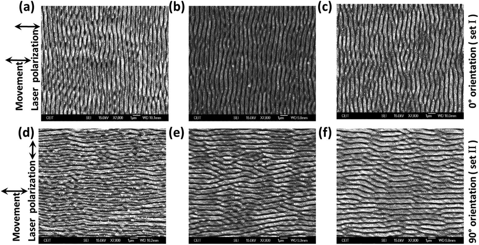
Figure 1.SEM images for quasi-sinusoidal LIPSS fabricated on top of a steel substrate using femtosecond laser processing. The polarization state of the laser beam is parallel to the direction of the movement during the sample processing for (a)–(c) subplots and perpendicular for (d)–(f).

Figure 2.(a) AFM image and profile for the sample with period $P = 631 nm$ from set I. (b) AFM image and profile for the sample with period $P = 606 nm$ from set II.

The profile is strongly dependent on the material of the sample, the conditions of the surface [34 –37], and even on the substrate temperature [38,39]. This means that this profile departs from the ideal sinusoidal form. To accurately fit the simulated results of the optical polarization parameters with the experimental values, we need to take this deformation into account by introducing the profile function $h (x) = \frac{GH}{2} {1 - 2 {[\frac{1 + \cos (2 π x / P)}{2}]}^{β}},$ (1)where $h (x)$ represents the height at each point along the $x$ –axis in the simulated periodic unit cell, GH is the profile height, and $P$ is the period. When the parameter $β$ is equal to 1, we obtain the ideal sinusoidal shape geometry, as shown at the top of Fig. 3(a). By changing $β$ we can simulate a flatter profile [ $β > 1$ , as shown on the bottom of Fig. 3(a)], or a sharper one [ $β < 1$ , as shown in the middle of Fig. 3(a)]. The geometrical parameters of the profile are also shown in Fig. 3(c) for the sinusoidal case treated in this section and for the binary profile shown in Fig. 3(b). The analysis made in this section, described by Eq. (1), uses $P = BW + S$ , where $S$ is the separation between grating elements, and BW is the width of the base of the sinusoidal profile.

Figure 3.Subwavelength gratings studied: (a) sinusoidal and (b) binary. They have a period $P = 632 nm$ and are made of stainless steel. (c) Transversal sections showing the geometrical parameters of the profiles. In subplot (a), we have included a graphic layout showing the vector and components of the incoming electric field $E$ , the azimuth angle $φ$ (in our case $φ = 45 °$ ), the wavevector $k$ , and the $X Y Z$ coordinate system. Note that the incidence angle is $α = 0 °$ and it is not represented.

Our model uses a plane wave impinging perpendicularly on the substrate, which is $α = 0 °$ in Fig. 3, and linearly polarized with its electric field oriented at an angle of $φ = 45 °$ , with respect to the $x$ –axis, and with an amplitude of $(1 / \sqrt{2},1 / \sqrt{2},0)$ in V/m. The grating is aligned along the $y$ –axis and the propagation is along the $z$ –direction, which is perpendicular to the substrate. The wavelength in the simulation, $λ = 633 nm$ , is the same as the experimental measurement. The optical field distribution along the whole structure has been calculated using the COMSOL Multiphysics simulation package. The unit cell used in the model has an air layer on top, and a substrate layer (steel) at the bottom, as shown in Fig. 3. The air domain is terminated with a perfectly matched layer (PML) on top that simulates a semi-infinite domain. The interface has a shape defined by Eq. (1) and is defined as a dedicated layer with a height equal to GH. The source is located on top of the air domain with its wavevector pointing toward the substrate. The index of refraction of stainless steel is obtained experimentally at $λ = 633 nm$ as ${\tilde{n}}_{steel} = 2.33 + 3.3 i$ . To represent the LIPSS structure, we replicate the previously defined unit cell transversely by applying Floquet periodic boundary conditions in the $X$ and $Y$ directions.

This analysis uses the Stokes vector to describe the state of polarization of the reflected light $S = (I, Q, U, V)$ [40], where $I$ is the intensity of the beam, $Q$ and $U$ represent the balance in power between horizontal and vertical axial polarizations, and linearly polarized (LP) light components at $45 °$ and $- 45 °$ , respectively. Finally, $V$ represents the balance between the right and left circular polarization (CP) components. These parameters obey the relation $I \geq \sqrt{Q^{2} + U^{2} + V^{2}}$ , being the equality condition applicable only for pure polarized beams. A normalized version of these parameters can be obtained just by dividing each one by the intensity $I$ . Then, the Stokes vector becomes $s = (1, q, u, v)$ and the relation among them becomes $1 \geq \sqrt{q^{2} + u^{2} + v^{2}}$ . In the case described in this section, as far as we assume a perfect 1D grating, these parameters comply with the pure polarization state condition $\sqrt{q^{2} + u^{2} + v^{2}} = 1$ .

The Stokes parameters of the light reflected by the fabricated structures were measured using an illumination spot of around 2 mm in diameter. The light source was a He–Ne laser [model 1122P, JDS Uniphase (JDSU), which is now VIAVI Solutions] emitting at $λ = 633 nm$ , with an spectral width lower than 0.002 nm.

The electric field distributions evaluated by the COMSOL software are used to calculate the Stokes parameters of the reflected light [33,40]. For each sample, the matching between experimental and simulated Stokes parameters is obtained individually by changing the geometry of the grating in terms of its height, GH, and shape $β$ [see Eq. (1)]. The result of this fitting is shown in Figs. 4(a) and 4(b), respectively. The simulated values for the Stokes parameters are represented by solid color lines, while the experimental values are represented by colored symbols.

Figure 4.Fitting of the simulated (solid lines) and experimentally measured (symbols) Stokes parameters for samples fabricated using femtosecond laser ablation with polarization (a) parallel and (b) perpendicular to the direction of the movement during the sample fabrication. (c)–(f) Plots show the geometrical parameters GH and $β$ of the profile that best fit the experimental data for the two sets of samples [set I in (c) and (e), and set II in (d) and (f)]. The dashed red circles select the lowest $β$ value on plot (e), and the highest $β$ value on plot (f). The solid lines in plots (c)–(f) represent the cubic polynomial fitting of the geometrical parameters versus $P$ .

The values of GH producing a best fitting are presented in Figs. 4(c), and 4(d), for sets I and II, respectively. The mean heights for sets I and II are ${GH}_{sim} = 140 \pm 10 nm$ and $147.5 \pm 5 nm$ , respectively. These values are close to the experimental mean value, which is ${GH}_{\exp} = 125 \pm 7 nm$ . The shape parameter $β$ that produces the best fitting is presented in Figs. 4(e) and 4(f) for sets I and II, respectively. The polarization parameters of set I fit better with sharper profiles than set II, meaning that set II seems to have a flatter top portion in the profile. The red dashed circles in Figs. 4(e) and 4(f) correspond to the lowest and highest $β$ values. These two points on the $β$ plots are for the samples measured by AFM, as shown by the images in Fig. 2. The profile has a sharper sinusoidal shape in Fig. 2(a), which corresponds to the point highlighted by the red dashed circle in Fig. 4(e). A flat-top profile of the LIPSS is obtained in Fig. 2(b), which corresponds to the point highlighted by the red dashed circle on Fig. 4(f). In both cases, the experimental profile images agree with the simulated values for the deformation. The SEM and AFM images show a structure with a localized periodicity that varies along the samples, where the top edges do not have a uniform profile. In this case, the values obtained from the simulation can be considered as the overall average for periodicity $P$ , height GH, and top edge deformation $β$ . From these results, we see how the optical model is able to accurately predict the optical response of a nonuniform LIPSS.

3. POLARIZATION MODULATION WITH BINARY AND SINUSOIDAL GRATINGS

To better understand the effect of the geometry of our LIPSS on the modification of the polarization state, besides the sinusoidal profile, we extend our calculations to binary gratings. These binary shapes are parameterized by the height of the profile, GH, and the width of the base, BW. In this section, we focus on how these geometrical parameters change the polarization state of the incoming light. We fix the period in both structures to $P = 632 nm$ , which lies within the range of the fabricated ones. Actually, this value can be tuned by changing the fabrication conditions [41,42]. We have used the same modeling setup used in the previous section, to conduct the calculation for this section. We move our analysis to $λ = 808 nm$ , ${\tilde{n}}_{steel} = 2.68 + 3.77 i$ , because the customized polarizers are important in near-IR spectroscopy [43]. The power performance of the LIPSS is described by the value of the reflectance. Here, remember that the transmittance of the system is zero, and the incoming power is distributed between reflected and absorbed power. As a consequence, a null reflectance is associated with filtering properties of the structure.

Figure 5 represents the normalized Stokes parameters $(q, u, v)$ of the reflected light and the reflectance as a function of the height GH and the base width BW for the binary profile (left) and the sinusoidal shape (right). In the case of the rectangular profile, BW can be related easily with the fill factor as $FF = BW / P$ . The sinusoidal shape is also characterized by the total height, GH, and by the distance between the minima of the profile, GW. The rest of the period not included within the BW range has a height equal to zero, meaning that the period of the sinusoidal grating has only one maximum. These calculations consider the shape parameter $β = 1$ . The geometrical parameters used in this section are also depicted in Fig. 3. The maps in Fig. 5 show some combinations of the geometrical parameters that generate maximum and minimum values of the Stokes parameters. In Fig. 5, we have also represented the reflectivity of the structure. These values should be compared to the reflectivity of a flat surface (no LIPSS) made of the same stainless steel, which is $R = 0.6$ .

Figure 5.Maps of the normalized Stokes parameters $q$ , $u$ , and $v$ , and reflectance $R$ , as a function of the geometrical parameters GH and BW for the binary (left) and sinusoidal (right) gratings. The maximum value of reflectivity $R_{\max} = 0.6$ is around the reflectivity value given by a regular, not nanostructured, stainless steel surface.

To have them properly identified, we label them with a capital letter: B for binary (rectangular) and $S$ for sinusoidal. Then, a subindex is added to denote the $q$ , $u$ , or $v$ parameters. Finally, a superscript is added as I, II, III, IV, V for the maximum or minimum number of locations, as shown on the maps of Fig. 5. The geometrical parameters for these locations are given in Table 1 for the binary and sinusoidal profiles.Table 1.

Geometrical Parameters and Reflectance of the Selected Minima and Maxima for the Binary and Sinusoidal Profiles^a

Binary Label	GH, BW [nm]	$R$ [%]	Pol. State	Sinusoidal Label	GH, BW [nm]	$R$ [%]	Pol. State
$B_{q}^{I}$	880, 275	12	90° LP	$S_{q}^{I}$	905, 615	23	90° LP
$B_{q}^{II}$	500, 300	19.3	90° LP	$S_{q}^{II}$	570, 620	17.6	90° LP
$B_{q}^{III}$	110, 375	28	90° LP	$S_{q}^{III}$	220, 625	31.1	90° LP
$B_{q}^{IV}$	615, 210	18	0° LP	$S_{q}^{IV}$	800, 350	14.5	0° LP
$B_{u}^{I}$	985, 200	16	$+ 45 °$ LP	$S_{u}^{I}$	995, 445	15.8	$- 45 °$ LP
$B_{u}^{II}$	580, 250	18.3	$+ 45 °$ LP	$S_{u}^{II}$	770, 440	17.5	$+ 45 °$ LP
$B_{u}^{III}$	245, 185	23.3	$+ 45 °$ LP	$S_{u}^{III}$	600, 360	39	$- 45 °$ LP
$B_{u}^{IV}$	500, 220	10.2	$- 45 °$ LP	$S_{u}^{IV}$	340, 295	59	$+ 45 °$ LP
$B_{u}^{V}$	940, 120	10.2	$- 45 °$ LP
$B_{v}^{I}$	640, 310	37.3	RCP	$S_{v}^{I}$	930, 420	8.7	RCP
$B_{v}^{II}$	250, 315	45.5	RCP	$S_{v}^{II}$	675, 400	18.7	LCP
$B_{v}^{III}$	540, 225	8.7	LCP	$S_{v}^{III}$	460, 380	32.2	RCP
$B_{v}^{IV}$	975, 155	12.4	LCP	$S_{v}^{IV}$	240, 165	46	LCP
$B_{v}^{V}$	200, 95	45.6	LCP

The state of polarization of the reflected light is given in the Pol. State column.

The identification of the maxima and minima in the maps of the Stokes parameters makes it possible to select geometrical parameters of the grating that generate a well-defined state of polarization. The maximum $q = 1$ corresponds to the horizontal linear polarization ( $0 ° LP$ ), and the minimum $q = - 1$ is for a vertical linear polarization ( $90 ° LP$ ). The maximum and minimum in $u$ ( $u = \pm 1$ ) are for $+ 45 ° LP$ and $- 45 ° LP$ , respectively. For the $v$ maps, we find the maxima $v = 1$ representing right-handed circular polarization (RCP); meanwhile the minima $v = - 1$ correspond to the left-handed circular polarization (LCP). A similar consequence can be extracted for the case of sinusoidal grating profiles, as shown in Figs. 5(b), 5(d), and 5(f). The corresponding reflectivity of the structure presented in Figs. 5(g) and 5(h) defines the geometrical parameters where the structure works as a filter (minimum reflectivity). A flat stainless steel substrate has a maximum reflectivity value of $R_{\max} = 0.6$ , which is about the same maximum obtained for the structure when including LIPSS, as shown in Figs. 5(g) and 5(h).

For the generated light states, we also calculated the azimuth angle $Ψ = 0.5 \arctan (\frac{U}{Q}),$ (2)and the ellipticity angle $χ = \arctan (\frac{V}{I + \sqrt{Q^{2} + U^{2}}}) .$ (3)

Azimuth directly represents the rotation angle of the axis of the polarization ellipse, allowing easy identification of the horizontal ( $Ψ = 0 °$ ), vertical ( $Ψ = 90 °$ ) and $\pm 45 °$ orientations of the polarization ellipse, as shown in Figs. 6(a) and 6(b). The ellipticity angle allows the easy identification of the linear ( $χ = 0 °$ ) and circular ( $χ = \pm 45 °$ ) polarization states, as shown in Figs. 6(c) and 6(d). It also shows how close an elliptical polarization state is of being linearly or circularly polarized. This combined analysis of the azimuth and ellipticity angles can be made using the contour lines presented in Fig. 6.

Figure 6.Maps of the azimuth $Ψ$ and ellipticity $χ$ angles as a function of BW and GH parameters for the binary (left column) and sinusoidal (right column) profiles. The contour lines in the azimuth maps represent the values of $Ψ = 45 °$ (in magenta), $Ψ = - 45 ° = 135 °$ (in cyan), and $Ψ = 0 °$ and $Ψ = 180 °$ (in yellow). The black contour lines in the ellipticity maps are for a value $χ = 0 °$ . The locations of the configurations with $χ = - 45 °$ and $χ = + 45 °$ are given as white dots in the blue and red regions, respectively.

The physical mechanisms of the polarization conversion may involve the selective absorption of the field components, and/or additional phase shifts between them. The input field components generate surface currents circulating the structure. Depending on the topography, these currents can be attenuated through Joule dissipation or plasmonic resonances, or they can emit electromagnetic waves with a phase difference between components that is strongly dependent on the geometry. The change in the polarization state can be visualized using 3D plots of the fields obtained by a full wave analysis of the structure during the propagation process. The results of this analysis are shown in Fig. 7 for the binary grating on the left, and sinusoidal on the right plots. The plots use a selection of some points in Table 1 to show representative polarization conversion using the binary or sinusoidal gratings. In Fig. 7(a), the locations of the source, LIPSS, reflected light, and PML domains are shown using yellow arrows. The reflected light can be axial LP, as in Figs. 7(a) and 7(b), or $\pm 45 ° LP$ , as in Figs. 7(c) and 7(d). Finally, the conversion from LP to CP light is shown in Fig. 7(e) for the LCP, and Fig. 7(f) for the RCP.

Figure 7.Full-wave propagation of the electric field on LIPSS for (a), (c), (e) binary grating, and (b), (d), (f) sinusoidal grating. The yellow arrows in (a) define the location of the source, LIPSS, reflection, and PML. The electric field in subplot (c) is linearly polarized and oriented along the 45° direction, being the point of view of the graphical representation almost coincident with the direction of the electric field vector. The labels for each field representation correspond to the cases presented in Table 1 and Fig. 5. We have also plotted the electric field distributions, along with the field evolution at the output, to help to understand the physical mechanism involved in the conversion.

The previous analysis is a particular case for just one incident illumination: 45° linearly polarized light. However, to totally characterize the polarimetric properties of the LIPSS, the polarization matrix of the material must be calculated. Since we assume that an LIPSS is periodical, depolarization analysis is not required, so we can use the Jones formalism. Mathematically, this is written as $E_{out} = P_{LIPSS} E_{in} = (\begin{matrix} E_{x, out} \\ E_{y, out} \end{matrix}) = (\begin{matrix} P_{x x} & P_{x y} \\ P_{y x} & P_{y y} \end{matrix}) (\begin{matrix} E_{x, in} \\ E_{y, in} \end{matrix}) .$ (4)

In our case, the grating generated as an LIPSS can be described by the corresponding Jones matrix $P_{LIPSS}$ and the input and output vectors $E_{in}$ and $E_{out}$ , which describe the incident and reflected light beams, respectively. Since the coordinate axis is aligned with the axis of the grating, the matrix becomes diagonal, meaning that $P_{x y} = P_{y x} = 0$ . Under these conditions, $P_{LIPSS} = (\begin{matrix} | P_{x x} | & 0 \\ 0 & | P_{y y} | e^{i ϕ} \end{matrix}) .$ (5)

Then, it is possible to obtain the two nonzero elements of the Jones matrix by just comparing the input and output electric field components: $| P_{x x} | = | E_{x, out} / E_{x, in} |,$ (6) $| P_{y y} | = | E_{y, out} / E_{y, in} |,$ (7) $ϕ = angle (E_{y, out}) - angle (E_{x, out}) .$ (8)

The reflectance of the LIPSS also can be calculated as $R = \frac{1}{2} ({| P_{x x} |}^{2} + {| P_{y y} |}^{2}) .$ (9)

Finally, we calculated these parameters from the simulations shown previously. Figure 8 represents the modulus of $P_{x x}$ and $P_{y y}$ , and the relative phase difference $φ$ between the components of the reflected electric field for both the rectangular profile (left column) and the sinusoidal profile (right column). These maps are given as a function of the geometric parameters GH and BW of the binary (rectangular) and sinusoidal profile. With Eq. (9), we obtain the maps of the reflectance given in Figs. 5(g) and 5(h). The minimum values obtained in $| P_{x x} |$ and $| P_{y y} |$ for the rectangular profile determine the geometrical configuration that generates a linear polarization state along the $y$ –axis and $x$ –axis, respectively. We can also look for the geometrical configurations with an equal value of the two diagonal elements $P_{x x} = P_{y y}$ and producing a phase shift $ϕ = \pm π / 2$ , because these configurations will generate circularly polarized waves. To obtain these configurations, we have plotted a yellow line on the phase shift map that represents the cases where $| P_{x x} | = | P_{y y} |$ , a blue circle for $ϕ = - π / 2$ , and an orange circle for $ϕ = + π / 2$ . These locations are the ones where the LIPSS behaves as a quarter-wave retarder. The Jones analysis shows that, by a proper selection of the geometry and orientation of an LIPSS, it can transform any pure state of polarization into any other.

Figure 8.Maps of the modulus of the elements of the Jones matrix $| P_{x x} |$ and $| P_{y y} |$ , and the relative phase shift between the electric field components of the reflected wave $ϕ$ , in terms of the geometrical parameters GH and BW. The left column is for the binary profile and the right column is for the sinusoidal shape. The yellow line in the phase map corresponds to the configuration that shows an equal value of the modulus of the diagonal elements of the Jones matrix. The dots are the locations on the $P_{x x} = P_{y y}$ line, where $ϕ = \pm π / 2$ ; i.e., the geometries for CP. These dots coincide with those presented in Figs. 6(c) and 6(d).

4. CONCLUSIONS

We show how a fabricated stainless steel LIPSS can produce a change in the state of polarization of an incoming radiation under normal incidence conditions. The Stokes parameters of several experimental samples with different periods and heights have been measured. These results have been compared to simulations obtained from computational electromagnetism. The shape of the LIPSS has been tuned to match the simulations to the experimental results. The resulting parameters for the fitting are in accordance with the experimental profiles derived from the SEM and AFM images.

Once the simulation conditions were validated, we made a detailed analysis of the LIPSS geometry for binary and sinusoidal shapes to find those configurations that generate a significant variation of the state of polarization of the incoming light. By controlling the steel nanostructure geometry, we can tune the polarization characteristics. These devices can act as wave retarders or linear polarizers. In fact, we have demonstrated that a customized profile of an LIPSS can generate any polarization state when illuminated by a linearly polarized beam having an azimuth of 45°. To summarize, we conclude that the analysis made here can promote the use of an LIPSS on stainless steel to fabricate low-cost retarders and polarization filters.

References

[1] Y. P. Svirko, N. I. Zheludev. Polarization of Light in Nonlinear Optics(2000).

[2] D. F. Eaton. Nonlinear optical materials. Science, 253, 281-287(1991).

[3] V. Lucarini, J. J. Saarinen, K.-E. Peiponen, E. M. Vartiainen. Kramers-Kronig Relations in Optical Materials Research, 110(2005).

[4] M. K. Chen, Y. Wu, L. Feng, Q. Fan, M. Lu, T. Xu, D. P. Tsai. Principles, functions, and applications of optical meta-lens. Adv. Opt. Mater., 9, 2001414(2021).

[5] M. B. Ross, C. A. Mirkin, G. C. Schatz. Optical properties of one-, two-, and three-dimensional arrays of plasmonic nanostructures. J. Phys. Chem. C, 120, 816-830(2016).

[6] J. Alda, G. D. Boreman. Infrared Antennas and Resonant Structures(2017).

[7] J. Zhou, L. J. Guo. Transition from a spectrum filter to a polarizer in a metallic nano-slit array. Sci. Rep., 4, 3614(2014).

[8] L. Wang, Z. Zhang. Resonance transmission or absorption in deep gratings explained by magnetic polaritons. Appl. Phys. Lett., 95, 111904(2009).

[9] C. Han, W. Y. Tam. Plasmonic ultra-broadband polarizers based on Ag nano wire-slit arrays. Appl. Phys. Lett., 106, 081102(2015).

[10] C. Lertvachirapaiboon, A. Baba, S. Ekgasit, K. Shinbo, K. Kato, F. Kaneko. Transmission surface plasmon resonance techniques and their potential biosensor applications. Biosens. Bioelectron., 99, 399-415(2018).

[11] A. Polyakov, K. Thompson, S. Dhuey, D. Olynick, S. Cabrini, P. Schuck, H. Padmore. Plasmon resonance tuning in metallic nanocavities. Sci. Rep., 2, 933(2012).

[12] M. Vincenti, D. de Ceglia, M. Grande, A. D’Orazio, M. Scalora. Tailoring absorption in metal gratings with resonant ultrathin bridges. Plasmonics, 8, 1445-1456(2013).

[13] H. Yan, L. Huang, X. Xu, S. Chakravarty, N. Tang, H. Tian, R. T. Chen. Unique surface sensing property and enhanced sensitivity in microring resonator biosensors based on subwavelength grating waveguides. Opt. Express, 24, 29724-29733(2016).

[14] N. Kazanskiy, M. Butt, S. Khonina. Silicon photonic devices realized on refractive index engineered subwavelength grating waveguides-a review. Opt. Laser Technol., 138, 106863(2021).

[15] P. Dong, Y. Wu, W. Guo, J. Di. Plasmonic biosensor based on triangular Au/Ag and Au/Ag/Au core/shell nanoprisms onto indium tin oxide glass. Plasmonics, 8, 1577-1583(2013).

[16] D. V. Nesterenko, Z. Sekkat. Resolution estimation of the Au, Ag, Cu, and Al single-and double-layer surface plasmon sensors in the ultraviolet, visible, and infrared regions. Plasmonics, 8, 1585-1595(2013).

[17] P. R. West, S. Ishii, G. V. Naik, N. K. Emani, V. M. Shalaev, A. Boltasseva. Searching for better plasmonic materials. Laser Photon. Rev., 4, 795-808(2010).

[18] L. Polavarapu, L. M. Liz-Marzán. Towards low-cost flexible substrates for nanoplasmonic sensing. Phys. Chem. Chem. Phys., 15, 5288-5300(2013).

[19] M. Seo, J. Lee, M. Lee. Grating-coupled surface plasmon resonance on bulk stainless steel. Opt. Express, 25, 26939-26949(2017).

[20] M. S. Ahsan, F. Ahmed, Y. G. Kim, M. S. Lee, M. B. Jun. Colorizing stainless steel surface by femtosecond laser induced micro/nano-structures. Appl. Surf. Sci., 257, 7771-7777(2011).

[21] T.-F. Yao, P.-H. Wu, T.-M. Wu, C.-W. Cheng, S.-Y. Yang. Fabrication of anti-reflective structures using hot embossing with a stainless steel template irradiated by femtosecond laser. Microelectron. Eng., 88, 2908-2912(2011).

[22] P. Boillot, J. Peultier. Use of stainless steels in the industry: recent and future developments. Proc. Eng., 83, 309-321(2014).

[23] L. Chi. Nanotechnology, 8(2010).

[24] J. Bonse, A. Rosenfeld, J. Krüger. On the role of surface plasmon polaritons in the formation of laser-induced periodic surface structures upon irradiation of silicon by femtosecond-laser pulses. J. Appl. Phys., 106, 104910(2009).

[25] A. Y. Vorobyev, C. Guo. Direct femtosecond laser surface nano/microstructuring and its applications. Laser Photon. Rev., 7, 385-407(2013).

[26] M. Birnbaum. Semiconductor surface damage produced by ruby lasers. J. Appl. Phys., 36, 3688-3689(1965).

[27] M. J. Cherukara, K. Sasikumar, A. DiChiara, S. J. Leake, W. Cha, E. M. Dufresne, T. Peterka, I. McNulty, D. A. Walko, H. Wen, S. J. R. S. Sankaranarayanan, R. J. Harder. Ultrafast three-dimensional integrated imaging of strain in core/shell semiconductor/metal nanostructures. Nano Lett., 17, 7696-7701(2017).

[28] C. Byram, S. S. B. Moram, A. K. Shaik, V. R. Soma. Versatile gold based SERS substrates fabricated by ultrafast laser ablation for sensing picric acid and ammonium nitrate. Chem. Phys. Lett., 685, 103-107(2017).

[29] A. Y. Zhizhchenko, P. Tonkaev, D. Gets, A. Larin, D. Zuev, S. Starikov, E. V. Pustovalov, A. M. Zakharenko, S. A. Kulinich, S. Juodkazis, A. A. Kuchmizhak, S. V. Makarov. Light-emitting nanophotonic designs enabled by ultrafast laser processing of halide perovskites. Small, 16, 2000410(2020).

[30] M. Sanz, M. Lopez-Arias, J. F. Marco, R. de Nalda, S. Amoruso, G. Ausanio, S. Lettieri, R. Bruzzese, X. Wang, M. Castillejo. Ultrafast laser ablation and deposition of wide band gap semiconductors. J. Phys. Chem. C, 115, 3203-3211(2011).

[31] A. Rudenko, J.-P. Colombier, S. Höhm, A. Rosenfeld, J. Krüger, J. Bonse, T. E. Itina. Spontaneous periodic ordering on the surface and in the bulk of dielectrics irradiated by ultrafast laser: a shared electromagnetic origin. Sci. Rep., 7, 12306(2017).

[32] A. Cerkauskaite, R. Drevinskas, A. Solodar, I. Abdulhalim, P. G. Kazansky. Form-birefringence in ITO thin films engineered by ultrafast laser nanostructuring. ACS Photon., 4, 2944-2951(2017).

[33] A. San-Blas, M. Martinez-Calderon, J. Buencuerpo, L. M. Sanchez-Brea, J. Del Hoyo, M. Gómez-Aranzadi, A. Rodríguez, S. Olaizola. Femtosecond laser fabrication of LIPSS-based waveplates on metallic surfaces. Appl. Surf. Sci., 520, 146328(2020).

[34] J. Sipe, J. F. Young, J. Preston, H. Van Driel. Laser-induced periodic surface structure. I. Theory. Phys. Rev. B, 27, 1141-1154(1983).

[35] A. Vorobyev, C. Guo. Enhanced absorptance of gold following multipulse femtosecond laser ablation. Phys. Rev. B, 72, 195422(2005).

[36] C. Florian, S. V. Kirner, J. Krüger, J. Bonse. Surface functionalization by laser-induced periodic surface structures. J. Laser Appl., 32, 022063(2020).

[37] M. Prudent, F. Bourquard, A. Borroto, J.-F. Pierson, F. Garrelie, J.-P. Colombier. Initial morphology and feedback effects on laser-induced periodic nanostructuring of thin-film metallic glasses. Nanomaterials, 11, 1076(2021).

[38] S. Gräf, C. Kunz, S. Engel, T. J.-Y. Derrien, F. A. Müller. Femtosecond laser-induced periodic surface structures on fused silica: the impact of the initial substrate temperature. Materials, 11, 1340(2018).

[39] Q. Li, Q. Wu, Y. Li, C. Zhang, Z. Jia, J. Yao, J. Sun, J. Xu. Femtosecond laser-induced periodic surface structures on lithium niobate crystal benefiting from sample heating. Photon. Res., 6, 789-793(2018).

[40] E. Collett. Field Guide to Polarization(2005).

[41] E. Skoulas, A. Manousaki, C. Fotakis, E. Stratakis. Biomimetic surface structuring using cylindrical vector femtosecond laser beams. Sci. Rep., 7, 45114(2017).

[42] N. Livakas, E. Skoulas, E. Stratakis. Omnidirectional iridescence via cylindrically-polarized femtosecond laser processing. Opto-Electron. Adv., 3, 190035(2020).

[43] H. W. Siesler, Y. Ozaki, S. Kawata, H. M. Heise. Near-infrared Spectroscopy: Principles, Instruments, Applications(2008).