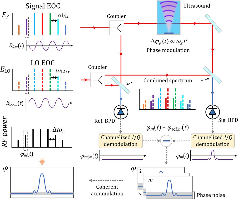
Fig. 1. Schematic for the concept of DCMHI.

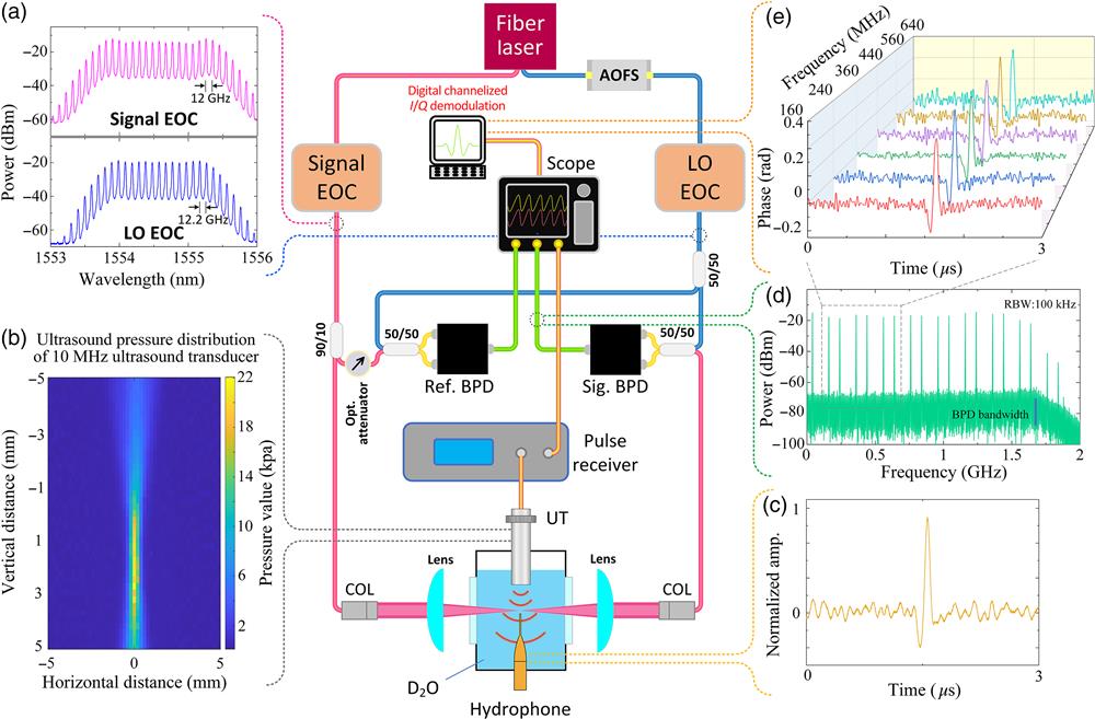
Fig. 2. Experimental demonstration of the DCMHI for detecting the ultrasound. EOC, electro-optics frequency comb; AOFS, acoustic-optics frequency shifter; COL, collimator; BPD, balanced photodiode; and UT, ultrasound transducer. (a) The optical spectrum of the signal EOC (red) and the LO EOC (blue). (b) The ultrasound distribution of the 10 MHz ultrasound transducer measured by hydrophone. (c) The ultrasound signal generated by the ultrasound transducer in the time domain. (d) The beat notes of dual-EOCs measured by the spectrum analyzer. (e) The demodulated phase values of different beat notes by channelized $I/Q$ demodulation from the recorded time domain signals.

Fig. 3. (a) The comparison diagram of demodulated phase values of the first-order comb tone ($m=1$) and synthesized 4 comb tones ($m=1$ to 4) in the time domain. (b) The accumulated phase SNR values with the respective standard deviations indicated as error bars, which are demodulated values collected ten times.

Fig. 4. The measured phase values of synthesized six comb tones in the DCMHI as a function of acoustic pressure; the solid line is the linear fit, and dots are measured data. The error bars on measured data are standard deviations after 10 measurements.

Fig. 5. The measured RMS NEP under different acoustic frequencies. Insets show segments extracted from the different sampled waveforms (original length is $20\mu \mathrm{s}$). The vertical axis is the respective normalized amplitude value. The dash shows the trend of NEP increasing with the demodulation bandwidth.

Fig. 6. The measured frequency response of the DCMHI. The inset demonstrates the relative response of the 1 MHz transducer measured by the DCMHI and hydrophone, respectively.

Fig. 7. Instantaneous ultrasonic pressure distribution (Video 1, MP4, 649 KB [URL: https://doi.org/10.1117/1.APN.2.1.016002.s1]).

Fig. 8. Instantaneous ultrasonic pressure distribution with positive and negative pressure changes (Video 2, MP4, 3.05 MB [URL: https://doi.org/10.1117/1.APN.2.1.016002.s2]).

Table 1. Setting parameters in the NEP measurement.

Table 2. Summary of the performances of the optical ultrasonic detectors.