• Photonics Research
  • Vol. 11, Issue 2, 150 (2023)
Lin Jiao and Jun-Hong An*
Author Affiliations
  • Lanzhou Center for Theoretical Physics, Key Laboratory of Theoretical Physics of Gansu Province, Lanzhou University, Lanzhou 730000, China
  • show less
    DOI: 10.1364/PRJ.469779 Cite this Article Set citation alerts
    Lin Jiao, Jun-Hong An. Noisy quantum gyroscope[J]. Photonics Research, 2023, 11(2): 150 Copy Citation Text show less
    (a) Schematic diagram of quantum gyroscope. (b) Evolution of the error δΩBA (cyan solid line) in the presence of photon loss under the Born–Markovian approximation. The blue dashed line is the local minima of δΩBA. The global minimum is marked by the red dot. (c) Numerical fitting reveals that the global minimum scales with the photon number as minδΩBA=5.4κN−0.23. The parameters are N=100, Ω=ω0, and κ=0.2ω0.
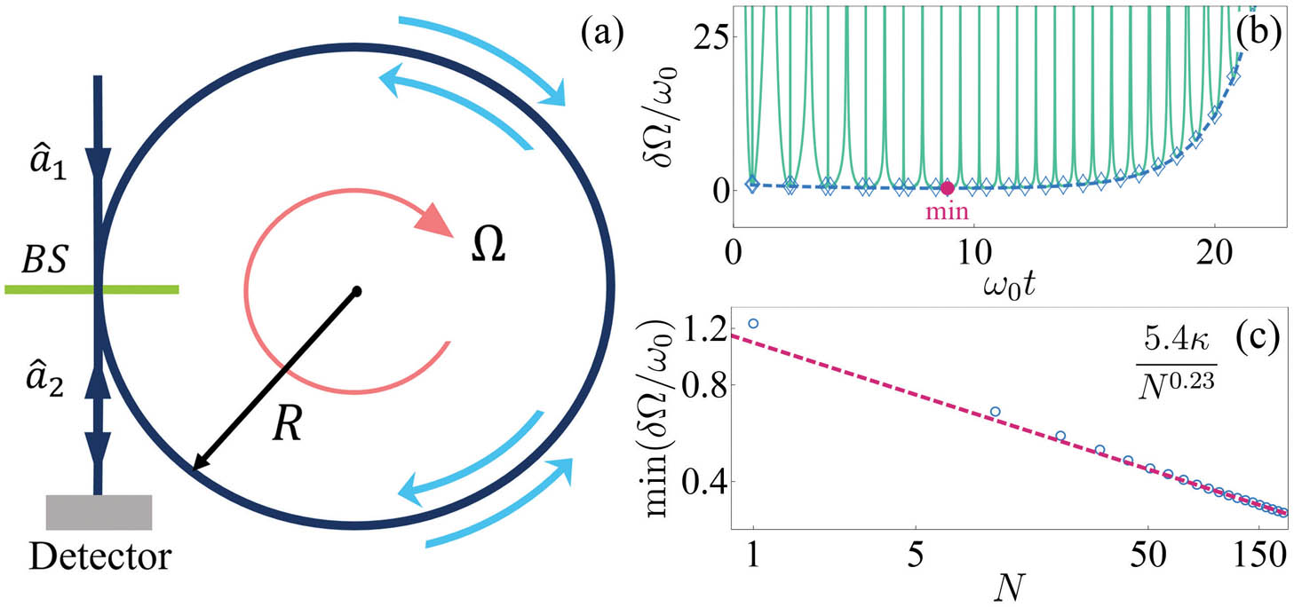
    Fig. 1. (a) Schematic diagram of quantum gyroscope. (b) Evolution of the error δΩBA (cyan solid line) in the presence of photon loss under the Born–Markovian approximation. The blue dashed line is the local minima of δΩBA. The global minimum is marked by the red dot. (c) Numerical fitting reveals that the global minimum scales with the photon number as minδΩBA=5.4κN0.23. The parameters are N=100, Ω=ω0, and κ=0.2ω0.
    (a) Energy spectrum of the total system formed by the two optical fields and their environments. Non-Markovian dynamical evolution of δΩ(t) multiplied by a magnification factor P when (ωc/ω0,P)=(2,10−1) in (b), (20, 10−2) in (c), and (25, 10−3) in (d). The blue dashed line in (d) is obtained by numerically solving Eq. (5), and the cyan solid line is obtained from the analytical form Eq. (9). We use s=1, η=0.05, Ω=10−2ω0, and N=100.
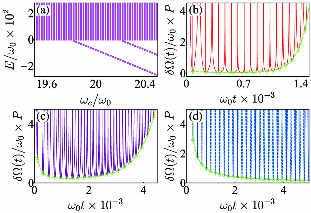
    Fig. 2. (a) Energy spectrum of the total system formed by the two optical fields and their environments. Non-Markovian dynamical evolution of δΩ(t) multiplied by a magnification factor P when (ωc/ω0,P)=(2,101) in (b), (20,102) in (c), and (25,103) in (d). The blue dashed line in (d) is obtained by numerically solving Eq. (5), and the cyan solid line is obtained from the analytical form Eq. (9). We use s=1, η=0.05, Ω=102ω0, and N=100.
    Local minima of δΩ(t) as a function of (a) time and (b) N when t=2.5×10⁴ω0−1 at different ωc. Steady-state |ul(∞)| marked by dots, which match with Zl depicted by lines, and the energy spectrum are shown in the inset of (b). We use s=1, η=7×10⁻⁴, Ω=10−2ω0, and N=100.
    Fig. 3. Local minima of δΩ(t) as a function of (a) time and (b) N when t=2.5×10⁴ω01 at different ωc. Steady-state |ul()| marked by dots, which match with Zl depicted by lines, and the energy spectrum are shown in the inset of (b). We use s=1, η=7×10⁴, Ω=102ω0, and N=100.
    Local minima of δΩ(t) as a function of (a) time and (b) N when t=2.5×10⁴ω0−1 at different η. Steady-state |ul(∞)| marked by dots, which match with Zl depicted by lines, and the energy spectrum are shown in the inset of (b). We use s=1, ωc=5×10³ω0, Ω=10−2ω0, and N=100.
    Fig. 4. Local minima of δΩ(t) as a function of (a) time and (b) N when t=2.5×10⁴ω01 at different η. Steady-state |ul()| marked by dots, which match with Zl depicted by lines, and the energy spectrum are shown in the inset of (b). We use s=1, ωc=5×10³ω0, Ω=102ω0, and N=100.
    (a)–(c) Solution of Eq. (C2) determined by the intersectors of two curves of y(E)=E (red dashed lines) and y(E)=Y+(E) (blue solid lines) or y(E)=Y−(E) (magenta dotted lines). In the regime E>0, both Y±(E) have infinite intersections with E, which form a continuous energy band. As long as either Y−(0)<0 or Y+(0)<0, an isolated eigenenergy corresponding to a bound state is formed in the regime E<0. (d)–(f) Corresponding behaviors of |u+(t)| (blue dotted lines) and |u−(t)| (red dashed lines) determined by numerically solving Eq. (A3). The light blue dotted and light red dashed lines in (d) and (e) show Zl determined by Eq. (C4). Accompanying the formation of a bound state, the corresponding |ul(t)| approaches a finite value, which exactly matches with Zl. The parameters are s=1, η=0.05, Ω=10−2ω0, ωc=2ω0 in (a) and (d), 20ω0 in (b) and (e), and 25ω0 in (c) and (f).
    Fig. 5. (a)–(c) Solution of Eq. (C2) determined by the intersectors of two curves of y(E)=E (red dashed lines) and y(E)=Y+(E) (blue solid lines) or y(E)=Y(E) (magenta dotted lines). In the regime E>0, both Y±(E) have infinite intersections with E, which form a continuous energy band. As long as either Y(0)<0 or Y+(0)<0, an isolated eigenenergy corresponding to a bound state is formed in the regime E<0. (d)–(f) Corresponding behaviors of |u+(t)| (blue dotted lines) and |u(t)| (red dashed lines) determined by numerically solving Eq. (A3). The light blue dotted and light red dashed lines in (d) and (e) show Zl determined by Eq. (C4). Accompanying the formation of a bound state, the corresponding |ul(t)| approaches a finite value, which exactly matches with Zl. The parameters are s=1, η=0.05, Ω=102ω0, ωc=2ω0 in (a) and (d), 20ω0 in (b) and (e), and 25ω0 in (c) and (f).
    (a) Global behavior of the local minima of the steady-state δΩ(t) as a function of N. (b) Threshold Nc in (a) as a function of Z1Z2. We use the same parameter values as the ones of the blue solid line in Fig. 4(b) of the main text.
    Fig. 6. (a) Global behavior of the local minima of the steady-state δΩ(t) as a function of N. (b) Threshold Nc in (a) as a function of Z1Z2. We use the same parameter values as the ones of the blue solid line in Fig. 4(b) of the main text.