Noisy quantum gyroscope

Lin Jiao; Jun-Hong An

doi:10.1364/PRJ.469779

Abstract

Gyroscope for rotation sensing plays a key role in inertial navigation systems. Developing more precise gyroscopes than the conventional ones bounded by the classical shot-noise limit by using quantum resources has attracted much attention. However, existing quantum gyroscope schemes suffer severe deterioration under the influence of decoherence, which is called the no-go theorem of noisy metrology. Here, by using two quantized optical fields as the quantum probe, we propose a quantum gyroscope scheme breaking through the constraint of the no-go theorem. Our exact analysis of the non-Markovian noise reveals that both the evolution time as a resource in enhancing the sensitivity and the achieved super-Heisenberg limit in the noiseless case are asymptotically recoverable when each optical field forms a bound state with its environment. The result provides a guideline for realizing high-precision rotation sensing in realistic noisy environments.

1. INTRODUCTION

High-performance gyroscopes for rotation sensing are of pivotal significance for navigation in many types of air, ground, marine, and space applications. Based on the Sagnac effect, i.e., two counter-propagating waves in a rotating loop accumulate a rotation-dependent phase difference, gyroscopes have been realized in optical [1 –6] and matter–wave [7 –14] systems. However, the precision of a purely Sagnac gyroscope, which is proportional to the surface area enclosed by the optical path, is theoretically limited by the classical shot-noise limit (SNL). It dramatically constrains their practical application and further performance improvement. The records for precision and stability of commercial gyroscopes are held by optical gyroscopes [15,16]. To reduce the noise effect, the practical operation of fiber optical gyroscopes generally modulates the optical signal and measures the ratios of harmonics instead of the phase difference [17], where the classical SNL model is not widely used. Building a purely Sagnac optical gyroscope beating the SNL from the fundamental principle is highly desired.

Pursuing more precise measurement to physical quantities than the classical SNL by using quantum resources [18 –22], such as squeezing [23 –25] and entanglement [26,27], quantum metrology supplies a way toward achieving gyroscopes with ultimate sensitivity limits. Based on this idea, many schemes of quantum gyroscopes have been proposed. It was found that the entanglement in N00N states [28,29], continuous-variable squeezing [30 –32], and optical nonlinearity [33] can enhance the sensitivity of optical gyroscopes beyond the SNL. A quantum-enhanced sensitivity can also be achieved in matter–wave gyroscopes [34 –37] by using spin squeezing [38 –40] or entanglement. However, quantum gyroscopes are still at the stage of the proof-of-principle study, and their superiority over the conventional ones in the absolute value of sensitivity still has not been exhibited [22,36]. One key obstacle is that the stability of the quantum gyroscope is challenged by the decoherence caused by inevitable noise in microscopic world, which generally makes the quantum resources degraded. It was found that the metrology sensitivity using entanglement [41 –43] and squeezing [44,45] exclusively returns to or even becomes worse than the SNL; thus, their quantum superiority completely disappears when the photon loss is considered. This is called the no-go theorem of noisy quantum metrology [46,47] and is one difficulty in achieving a high-precision quantum gyroscope in practice.

In this paper, we propose a scheme of quantum gyroscope and discover a mechanism to overcome the constraint of the no-go theorem on our scheme. A super-Heisenberg limit (HL) on the sensitivity is achieved in the ideal case by using two-mode squeezed vacuum state. Our exact analysis on the photon dissipation reveals that the performance of the quantum gyroscope in the dissipative environments intrinsically depends on the energy-spectrum feature of the total system formed by the probe and its environments. The encoding time as resource and the super-HL in the ideal case are asymptotically recovered when each optical field forms a bound state with its environment, which means that the no-go theorem is efficiently avoided. It supplies a guideline to engineer the optimal working condition of our quantum gyroscope in dissipative environments.

Sign up for Photonics Research TOC. Get the latest issue of Photonics Research delivered right to you！Sign up now

2. IDEAL QUANTUM GYROSCOPE SCHEME

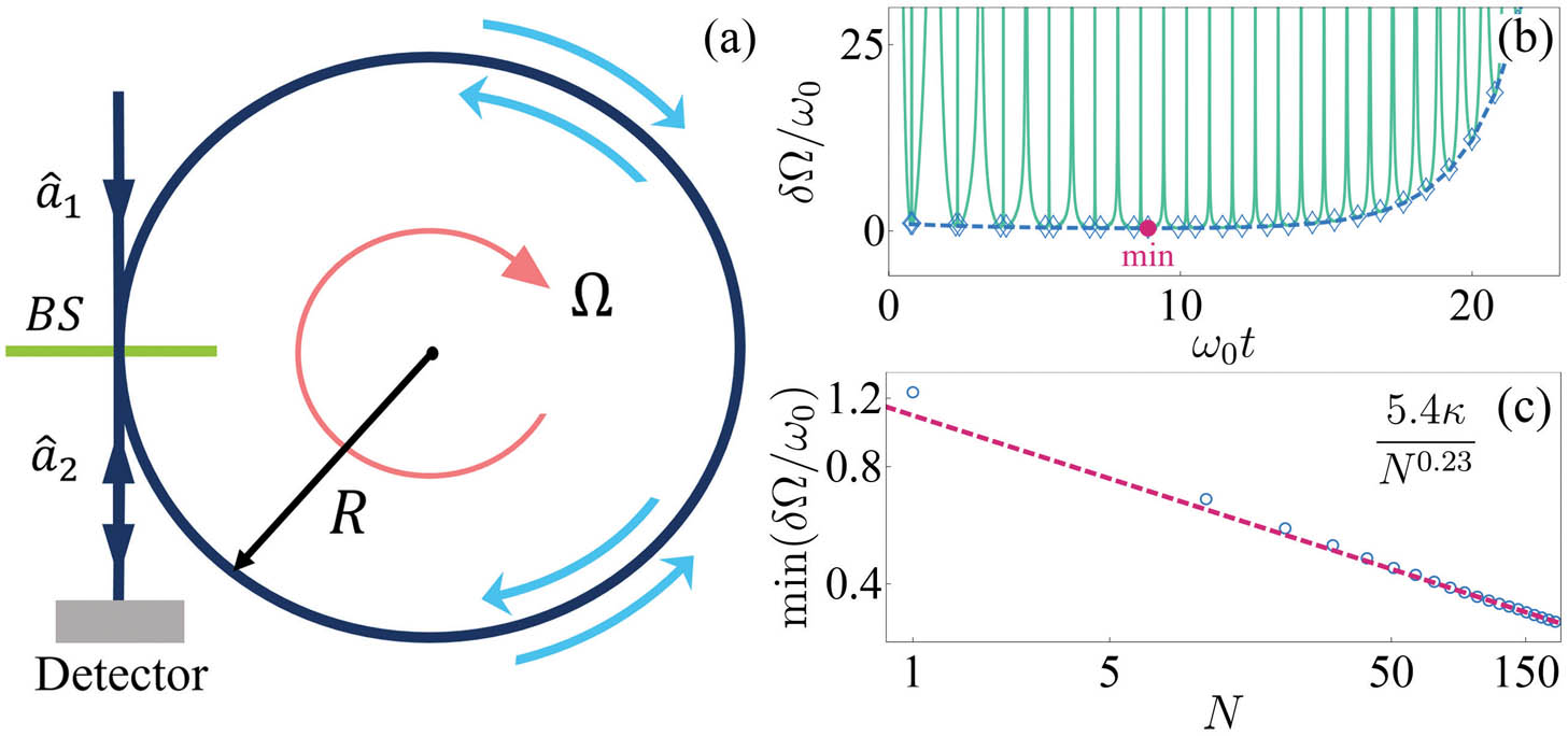
To measure a physical quantity of certain systems, three processes, i.e., the initialization of the quantum probe, the quantity encoding via the probe-system coupling, and the measurement, are generally required. In our quantum gyroscope, we choose two beams of quantized optical fields as the quantum probe. They propagate in opposite directions and are input into a 50:50 beam splitter and split into clockwise and counterclockwise prorogating beams [see Fig. 1(a)]. The setup rotates with an angular velocity $Ω$ about the axis perpendicular to its plane. Thus, the two beams accumulate a phase difference $Δ θ = N 4 π k R^{2} Ω / c$ when they reencounter the beam splitter after $N$ rounds of propagation in the circular path [48]. Here $k$ is the wave vector, $c$ is the speed of light, and $R$ is the radius of the quantum gyroscope. Remembering the standing-wave condition $k R = n$ ( $n \in Z$ ) of the optical fields propagating along the circular path and defining $Δ t \equiv N 2 π R / c$ , we have $Δ ω \equiv Δ θ / Δ t = 2 n Ω$ . Therefore, the quantum gyroscope can be equivalently treated as two counter-propagating optical fields with a frequency difference $Δ ω$ along the circular path. For concreteness, we choose the basic mode $n = 1$ . Then the optical fields in the quantum gyroscope can be quantum mechanically described by $(ℏ = 1)$ [49] ${\hat{H}}_{S} = ω_{0} \sum_{l = 1,2} {\hat{a}}_{l}^{†} {\hat{a}}_{l} + Ω ({\hat{a}}_{1}^{†} {\hat{a}}_{1} - {\hat{a}}_{2}^{†} {\hat{a}}_{2}),$ (1)where ${\hat{a}}_{l}$ is the annihilation operator of the $l$ th field with frequency $ω_{0}$ . The optical fields couple to the beam splitter twice and output in the state $| Ψ_{out} ⟩ = \hat{V} {\hat{U}}_{0} (Ω, t) \hat{V} | Ψ_{in} ⟩$ , where ${\hat{U}}_{0} (Ω, t) = \exp (- i {\hat{H}}_{S} t)$ is the evolution operator of the fields and $\hat{V} = \exp [i \frac{π}{4} ({\hat{a}}_{1}^{†} {\hat{a}}_{2} + {\hat{a}}_{2}^{†} {\hat{a}}_{1})]$ describes the action of the beam splitter. Thus, the angular velocity $Ω$ is encoded into the state $| Ψ_{out} ⟩$ of the optical probe via the unitary evolution.

Figure 1.(a) Schematic diagram of quantum gyroscope. (b) Evolution of the error $δ Ω_{BA}$ (cyan solid line) in the presence of photon loss under the Born–Markovian approximation. The blue dashed line is the local minima of $δ Ω_{BA}$ . The global minimum is marked by the red dot. (c) Numerical fitting reveals that the global minimum scales with the photon number as $\min δ Ω_{BA} = 5.4 κ N^{- 0.23}$ . The parameters are $N = 100$ , $Ω = ω_{0}$ , and $κ = 0.2 ω_{0}$ .

To exhibit the quantum superiority, we employ two-mode squeezed vacuum state as the input state $| Ψ_{in} ⟩ = \hat{S} | 0,0 ⟩$ , where $\hat{S} = \exp [r ({\hat{a}}_{1} {\hat{a}}_{2} - {\hat{a}}_{1}^{†} {\hat{a}}_{2}^{†})]$ is the squeezing operator, with $r$ being the squeezing parameter. The total photon number of this input state is $N = 2 \sinh^{2} r$ , which is the quantum resource of our scheme. The parity operator $\hat{Π} = \exp (i π {\hat{a}}_{1}^{†} {\hat{a}}_{1})$ is measured at the output port [50]. To the output state $| Ψ_{out} ⟩$ , we can calculate $\bar{Π} \equiv ⟨ Ψ_{out} | \hat{Π} | Ψ_{out} ⟩ = [1 + N (2 + N) \cos^{2} (2 Ω t {)]}^{- 1 / 2}$ and $δ Π = {(1 - {\bar{Π}}^{2})}^{1 / 2}$ , where ${\hat{Π}}^{2} = 1$ has been used. Then the sensitivity of sensing $Ω$ can be evaluated via the error propagation formula $δ Ω = \frac{δ Π}{| \partial_{Ω} \bar{Π} |}$ as $\min δ Ω = {[2 t \sqrt{N (2 + N)}]}^{- 1},$ (2)when $Ω t = (2 n + 1) π / 4$ with $n \in Z$ . It is remarkable to find that the best sensing error achieved in our scheme is even smaller than the HL $Δ Ω \propto {(t N)}^{- 1}$ , which reflects the quantum superiority of the used squeezing and measured observable in our scheme. It can be verified that this measurement scheme saturates the Cramér–Rao bound governed by quantum Fisher information. We call such a sensitivity surpassing the HL the super-HL [51,52]. It is noted that a phase estimation error smaller than the inverse of the mean photon number was called the sub-HL in Refs. [50,53,54]. The outstanding performance of quantum squeezing has been found in gravitational wave detection [55].

3. EFFECTS OF DISSIPATIVE ENVIRONMENTS

The superiority of the quantum sensor is challenged by the decoherence of the quantum probe due to the inevitable interactions with its environment. Depending on whether the probe has energy exchange with the environment or not, the decoherence can be classified into dissipation and dephasing. The main decoherence in our quantum gyroscope is the photon dissipation. The previous works phenomenologically treat the photon dissipation by introducing an imperfect transmission to the beam splitter [41,44,45,56,57], which is equivalent to the Born–Markovian approximate description. Such an approximation is convenient, but it might miss important physics. It has been found that the system–environment interplay caused by the inherent non-Markovian nature would induce diverse characters absent in the Born–Markovian approximation [58 –62]. To reveal the practical performance of our quantum gyroscope, we, going beyond the Born–Markovian approximation and paying special attention to the non-Markovian effect, investigate the impact of the photon dissipation on the scheme.

We consider that the encoding process is influenced by the photon dissipation, which is caused by the energy exchange between the two optical fields and two independent environments [48]. The Hamiltonian of the total system is $\hat{H} = {\hat{H}}_{S} + \sum_{l = 1,2} \sum_{k} [ω_{k, l} {\hat{b}}_{k, l}^{†} {\hat{b}}_{k, l} + g_{k, l} ({\hat{a}}_{l}^{†} {\hat{b}}_{k, l} + H .c .)],$ (3)where ${\hat{b}}_{k, l}$ is the annihilation operator of the $k$ th mode with frequency $ω_{k, l}$ of the environment felt by the $l th$ optical field and $g_{k, l}$ is their coupling strength. The coupling is further characterized by the spectral density $J_{l} (ω) = \sum_{k} g_{k, l}^{2} δ (ω - ω_{k})$ in the continuous limit of the environmental frequencies. We consider the Ohmic-family spectral density $J_{1} (ω) = J_{2} (ω) \equiv J (ω) = η ω^{s} ω_{c}^{1 - s} e^{- ω / ω_{c}}$ for both environments, where $η$ is a dimensionless coupling constant, $ω_{c}$ is a cutoff frequency, and $s$ is an Ohmicity index. Under the condition that the environments are initially in the vacuum state, we can derive an exact master equation for the encoding process using the Feynman–Vernon influence functional method [63], $\dot{ρ} (t) = \sum_{l = 1,2} {- i ϖ_{l} (t) [{\hat{a}}_{l}^{†} {\hat{a}}_{l}, ρ (t)] + γ_{l} (t) {\hat{D}}_{l} ρ (t)},$ (4)where ${\hat{D}}_{l} \cdot = 2 {\hat{a}}_{l} \cdot {\hat{a}}_{l}^{†} - {\hat{a}}_{l}^{†} {\hat{a}}_{l} \cdot - \cdot {\hat{a}}_{l}^{†} {\hat{a}}_{l}$ is the Lindblad superoperator, $ϖ_{l} (t) = - Im [{\dot{u}}_{l} (t) / u_{l} (t)]$ is the renormalized frequency, and $γ_{l} (t) = - Re [{\dot{u}}_{l} (t) / u_{l} (t)]$ is the dissipation rate. The time-dependent functions $u_{l} (t)$ satisfy ${\dot{u}}_{l} (t) + i ω_{l} u_{l} (t) + \int_{0}^{t} f (t - τ) u_{l} (τ) d τ = 0,$ (5)under $u_{l} (0) = 1$ , where $ω_{1,2} = ω_{0} \pm Ω$ and $f (x) = \int_{0}^{\infty} J (ω) e^{- i ω x} d ω$ is the environmental correlation function. Equation (4) indicates that all the non-Markovian effects induced by the environmental backactions have been incorporated into these time-dependent coefficients self-consistently. Solving Eq. (4), we obtain (see Appendix A) $\bar{Π} (t) = x [4 m_{1} (m_{2}^{*} - m_{1}^{*} p_{2}^{2}) + 4 m_{2} (m_{1}^{*} - m_{2}^{*} p_{1}^{2}) + {(1 - p_{1} p_{2})}^{2} + 16 {| m_{1} m_{2} |}^{2}]^{- 1 / 2},$ (6)where $x = {(\sqrt{A_{1} A_{2}} \cosh^{2} r)}^{- 1}$ , $m_{l} = \frac{- i u_{l} {(t)}^{2} \tanh r}{2 A_{l}}$ , and $p_{l} = | u_{l} (t {) |}^{2} (1 - A_{l}^{- 1})$ , with $A_{l} = 1 - {[| u_{l} (t {) |}^{2} - 1]}^{2} \tanh^{2} r$ . The analytical form of $δ Ω$ can then be calculated in a similar manner as the ideal case.

In the special case when the probe–environment coupling is weak and the time scale of $f (t - τ)$ is smaller than the typical time scale of the probe, we can apply the Born–Markovian approximation in Eq. (5) [41,57]. Their approximate solutions read $u_{l, BA} (t) = e^{- {κ_{l} + i [ω_{l} + Δ (ω_{l})]} t}$ , with $κ_{l} = π J (ω_{l})$ and $Δ (ω_{l}) = P \int_{0}^{\infty} \frac{J (ω)}{ω_{1} - ω} d ω$ . Substituting them into Eq. (6) and using the error propagation formula, we obtain (see Appendix B) $δ Ω_{BA} (t) = \frac{(2 e^{2 t κ} + N C e^{- 2 t κ}) \sqrt{C}}{\sqrt{8 N} (N + 2) t | \sin (4 Ω t) |},$ (7)where $C = 4 e^{2 t κ} + N - 2 + (N + 2) \cos (4 Ω t)$ . Here we have chosen $κ_{1} = κ_{2} \equiv κ$ . We plot in Fig. 1(b) the evolution of $δ Ω_{BA} (t)$ . It can be found that $δ Ω_{BA} (t)$ experiences an obvious oscillation with time. However, the best sensitivity manifested by the profile of its local minima tends to be divergent with time. Thus, being in sharp contrast to the ideal case in Eq. (2), the superiority of time as a resource in enhancing the precision of the quantum gyroscope disappears. After optimizing the encoding time, we obtain the global minimum $δ Ω$ [see the red dot in Fig. 1(b)]. The numerical fitting reveals $\min δ Ω = 5.4 κ N^{- 0.23}$ [see Fig. 1(c)], which is even worse than the SNL. Therefore, being consistent with the previous quantum sensing schemes [41,44,45,56,57], the photon dissipation under the Born–Markovian approximation makes the quantum advantages of our scheme completely vanish. It is called the no-go theorem of noisy quantum metrology [46,47] and is the main obstacle to achieve a high-precision quantum sensing in practice.

In the general non-Markovian case, the analytical solution of Eq. (5) can be found by the method of Laplace transform, which converts Eq. (5) into ${\tilde{u}}_{l} (z_{l}) = {[z_{l} + i ω_{l} + \int_{0}^{\infty} \frac{J (ω) d ω}{z_{l} + i ω} d ω]}^{- 1}$ . Then $u_{l} (t)$ is obtained by making the inverse Laplace transform to ${\tilde{u}}_{l} (z_{l})$ , which can be done by finding its poles from $Y_{l} (E_{l}) \equiv ω_{l} - \int_{0}^{\infty} \frac{J (ω)}{ω - E_{l}} d ω = E_{l}, E_{l} = i z_{l} .$ (8)Here, $E_{l}$ are also the eigenenergies in the single-excitation subspace of the total systems formed by each optical field and its environment. To see this, we expand the eigenstate as $| Φ_{l} ⟩ = (x_{l} {\hat{a}}_{l}^{†} + \sum_{k} y_{k, l} {\hat{b}}_{k, l}^{†} {) | 0, {0}_{k, l}} ⟩$ . From the stationary Schrödinger equation, we have $[E_{l} - (ω_{0} \pm Ω)] x_{l} = \sum_{k} g_{k, l} y_{k, l}$ and $y_{k, l} = ℏ g_{k, l} x_{l} / (E_{l} - ℏ ω_{k, l})$ with $E_{l}$ being the eigenenergies. The two equations readily result in Eq. (8) in the continuous limit of the environmental frequencies. It implies that the dissipation of the optical probe is intrinsically determined by the energy-spectrum character of the probe–environment system in the single-excitation subspace, even though the subspaces with any excitation numbers are involved. Due to $Y_{l} (E_{l})$ being decreasing functions in the regime $E_{l} < 0$ , each of Eq. (8) has one isolated root $E_{b, l}$ in this regime provided $Y_{l} (0) < 0$ . While $Y_{l} (E_{l})$ are ill-defined when $E_{l} > 0$ due to the poles in the integrand, they have infinite roots in this regime, which form a continuous energy band. We call the eigenstates of the isolated eigenenergies $E_{b, l}$ bound states [58]. Making the inverse Laplace transform, we obtain $u_{l} (t) = Z_{l} e^{- i E_{b, l} t} + \int_{0}^{\infty} Θ (E) e^{- i E t} d E$ , where $Z_{l} = {[1 + \int_{0}^{\infty} \frac{J (ω)}{{(E_{b, l} - ω)}^{2}} d ω]}^{- 1}$ and $Θ (E) = \frac{J (E)}{{[E - ω_{l} - Δ (E)]}^{2} + {[π J (E)]}^{2}}$ . The integral in $u_{l} (t)$ is from the energy band and tends to zero in the long-time limit due to the out-of-phase interference. Thus, when the bound state is formed, we have $\lim_{t \to \infty} u_{l} (t) = Z_{l} e^{- i E_{b, l} t}$ , characterizing the suppressed dissipation; otherwise, we have $\lim_{t \to \infty} u_{l} (t) = 0$ , meaning a complete dissipation. It can be determined that the bound state is formed for the Ohmic-family spectral density when $ω_{l} < η ω_{c} Γ (s)$ , where $Γ (s)$ is the Euler’s $Γ$ function.

We have three parameter regimes where zero, one, and two bound states are formed, respectively. It is natural to expect that $δ Ω$ in the former two regimes is qualitatively consistent with the Born–Markovian approximate result Eq. (7) due to the complete dissipation in either two or one optical field. Focusing on the case in the presence of two bound states and substituting the asymptotic solution $Z_{l} e^{- i E_{b, l} t}$ into Eq. (6), we obtain (see Appendix C) $\lim_{t \to \infty} δ Ω (t) = \frac{F \sqrt{2 F - 4}}{2 N (2 + N) Z_{1}^{2} Z_{2}^{2} t (Z_{1} + Z_{2}) | \sin (2 G t) |},$ (9)where $F = 2 + N \sum_{l} Z_{l}^{2} (2 - Z_{l}^{2}) + N Z_{1}^{2} Z_{2}^{2} [N + (2 + N) \cdot \cos (2 G t)]$ with $G = E_{b,1} - E_{b,2}$ . We have used $\partial_{Ω} E_{b, l} = (- {1)}^{l - 1} Z_{l}$ derived from Eq. (8). Equation (9) exhibits a $t^{- 1}$ -dependence on time, which is as perfect as the ideal result Eq. (2). Another finding from Eq. (9) is that it tends to the exactly same form as the ideal result Eq. (2) in the limit $Z_{l}$ tending to 1. Therefore, the formation of two bound states overcomes the problem of no-go theorem and asymptotically retrieves the ideal sensitivity.

4. NUMERICAL RESULTS

We now numerically verify our general result by choosing the Ohmic spectral density. Figure 2(a) shows the energy spectrum of the total system consisting of the optical fields and their environments. It can be seen that the two branches of bound states divide the energy spectrum into three regimes: without bound state when $ω_{c} < 19.8 ω_{0}$ , one bound state when $ω_{c} \in (19.8, 20.2) ω_{0}$ , and two bound states when $ω_{c} > 20.2 ω_{0}$ . The result confirms our analytical criterion that the bound states are formed when $ω_{c} > ω_{l} / [η Γ (s)]$ . Numerically solving Eq. (5) and using Eq. (6), we obtain the exact evolution of $δ Ω (t)$ in the three regimes. When no or one bound state is formed, the local minima profile of $δ Ω (t)$ tends to divergence in the long-time limit, and the quantum superiority of the scheme completely disappears [see Figs. 2(b) and 2(c)], which is qualitatively similar to the Born–Markovian result. However, as long as two bound states are formed, the profile of the local minima becomes a decreasing function of the encoding time. The matching of the numerical result with the long-time behavior Eq. (9) verifies the validity of the result in Eq. (9). Thus, the encoding time as a resource in sensing $Ω$ is recovered as perfectly as the ideal case by the formation of the two bound states. Our above result also gives a direct proof on that whether the Born–Markovian approximation is applicable or not depends sensitively on the feature of the energy spectrum of the total probe–environment system. Whenever a bound state is formed in the energy spectrum, the decoherence would be suppressed, and the Born–Markovian approximation would no long be valid anymore. This result refreshes our general belief on applicability of the Born–Markovian approximation.

Figure 2.(a) Energy spectrum of the total system formed by the two optical fields and their environments. Non-Markovian dynamical evolution of $δ Ω (t)$ multiplied by a magnification factor $P$ when $(ω_{c} / ω_{0}, P {) = (2, 10}^{- 1})$ in (b), $(20, 10^{- 2})$ in (c), and $(25, 10^{- 3})$ in (d). The blue dashed line in (d) is obtained by numerically solving Eq. (5), and the cyan solid line is obtained from the analytical form Eq. (9). We use $s = 1$ , $η = 0.05$ , $Ω {= 10}^{- 2} ω_{0}$ , and $N = 100$ .

Figure 3(a) shows the evolution of the local minima of $δ Ω (t)$ in Eq. (9) at different $ω_{c}$ when two bound states are formed. The formation of the bound state causes an abrupt increase of the corresponding $| u_{l} (\infty) |$ from zero to a finite value exactly matching with $Z_{l}$ [see the inset of Fig. 3(b)]. It is interesting to find that not only the encoding time as a resource is retrieved, but also the ideal precision is asymptotically recovered. This is double confirmed by the long-time behavior of $\min δ Ω (t)$ as a function of the photon number $N$ in Fig. 3(b). A similar performance is found by changing the coupling constant $η$ (see Fig. 4). All the results demonstrate the constructive role played by the two bound states and the non-Markovian effect in retrieving the quantum superiority of our quantum gyroscope. It offers us a guideline to achieve a noise-tolerant rotation sensing by manipulating the formation of the bound states. It is noted that, according to the condition of forming the bound states, we see that what really matters is the relative value $ω_{c} / ω_{0}$ . The equivalent result is achievable by tuning $ω_{0}$ for given $ω_{c}$ and $η$ .

Figure 3.Local minima of $δ Ω (t)$ as a function of (a) time and (b) $N$ when $t = 2.5 \times 10^{4} ω_{0}^{- 1}$ at different $ω_{c}$ . Steady-state $| u_{l} (\infty) |$ marked by dots, which match with $Z_{l}$ depicted by lines, and the energy spectrum are shown in the inset of (b). We use $s = 1$ , $η = 7 \times 10^{- 4}$ , $Ω {= 10}^{- 2} ω_{0}$ , and $N = 100$ .

Figure 4.Local minima of $δ Ω (t)$ as a function of (a) time and (b) $N$ when $t = 2.5 \times 10^{4} ω_{0}^{- 1}$ at different $η$ . Steady-state $| u_{l} (\infty) |$ marked by dots, which match with $Z_{l}$ depicted by lines, and the energy spectrum are shown in the inset of (b). We use $s = 1$ , $ω_{c} = 5 \times 10^{3} ω_{0}$ , $Ω {= 10}^{- 2} ω_{0}$ , and $N = 100$ .

5. DISCUSSION AND CONCLUSION

Our scheme is independent of the form of the spectral density. Although only the Ohmic form is considered, our scheme can be generalized to other spectra. Given the rich way of controlling the spectral density in the setting of quantum reservoir engineering [64,65], we deem that our scheme is realizable in state-of-the-art quantum-optical experiments. The Ohmic-family spectral densities for the electromagnetic noise are well cotrolled in circuit QED systems [66 –68]. Actually, the non-Markovian effect has been observed in the linear optical systems [69,70]. The bound state and its dynamical effect have been observed in circuit QED [71] and ultracold atom [72] systems. A squeezing parameter $r ≃ 2.5$ , which corresponds to $N ≃ 73$ , has been realized [73]. Inspired by these experimental achievements in circuit QED systems, we can design a realizable microwave Sagnac interferometer to test our result. We prepare two quantized optical fields propagating in opposite directions in a 1D transmission line, which is coupled via a capacitance or inductance to another wide-band transmission line acting as a structured environment [71]. The squeezed state of the two fields can be generated by the Josephson traveling-wave parametric amplifier [73]. When the fields reencounter after several rounds of rotation, a phase difference depending on the measured angular velocity is accumulated. The structured environments, on one hand, exert a strong non-Markovian effect on the dynamics of the fields and, on the other hand, protect the scheme from the photon loss according to our mechanism.

In summary, we have proposed a quantum gyroscope scheme by using two quantized fields as the quantum probe, which achieves a super-HL sensitivity in measuring the angular velocity. However, the photon dissipation under the conventional Born–Markovian approximation forces this sensitivity to even be worse than the classical SNL. To overcome this problem, we have presented a mechanism to retrieve the ideal sensitivity by relaxing this approximation. It is found that the ideal sensitivity is asymptotically recoverable when each optical field forms a bound state with its environment, which can be realized by the technique of quantum reservoir engineering. Exhibiting the optimal working condition of the quantum gyroscope, our mechanism breaks through the constraint of the no-go theorem of noisy quantum metrology and supplies a guideline for developing high-precision rotation sensing for next-generation inertial navigation systems.

APPENDIX A: EXPECTATION VALUE OF PARITY OPERATOR

ρ ({\bar{α}}_{f}, α_{f}^{'}; t) = \int d μ (α_{i}) d μ (α_{i}^{'}) J ({\bar{α}}_{f}, α_{f}^{'}; t | {\bar{α}}_{i}, α_{i}^{'}; 0) \times ρ ({\bar{α}}_{i}, α_{i}^{'}; 0),

| Ψ_{in} ⟩ = \exp [r ({\hat{a}}_{1} {\hat{a}}_{2} - {\hat{a}}_{1}^{†} {\hat{a}}_{2}^{†})] | 00 ⟩

u_{l} (t) = \exp (- i ω_{l} t)

APPENDIX B: SENSITIVITY UNDER THE BORN–MARKOVIAN APPROXIMATION

u_{l} (t) = e^{- i ω_{l} t} u_{l}^{'} (t)

u_{l, MA} (t)

APPENDIX C: SENSITIVITY IN THE NON-MARKOVIAN DYNAMICS

{\tilde{u}}_{l} (z_{l}) = {[z_{l} + i ω_{l} + \int_{0}^{\infty} \frac{J (ω) d ω}{z_{l} + i ω} d ω]}^{- 1}

Figure 5.(a)–(c) Solution of Eq. (C2) determined by the intersectors of two curves of $y (E) = E$ (red dashed lines) and $y (E) = Y_{+} (E)$ (blue solid lines) or $y (E) = Y_{-} (E)$ (magenta dotted lines). In the regime $E > 0$ , both $Y_{\pm} (E)$ have infinite intersections with $E$ , which form a continuous energy band. As long as either $Y_{-} (0) < 0$ or $Y_{+} (0) < 0$ , an isolated eigenenergy corresponding to a bound state is formed in the regime $E < 0$ . (d)–(f) Corresponding behaviors of $| u_{+} (t) |$ (blue dotted lines) and $| u_{-} (t) |$ (red dashed lines) determined by numerically solving Eq. (A3). The light blue dotted and light red dashed lines in (d) and (e) show $Z_{l}$ determined by Eq. (C4). Accompanying the formation of a bound state, the corresponding $| u_{l} (t) |$ approaches a finite value, which exactly matches with $Z_{l}$ . The parameters are $s = 1$ , $η = 0.05$ , $Ω {= 10}^{- 2} ω_{0}$ , $ω_{c} = 2 ω_{0}$ in (a) and (d), $20 ω_{0}$ in (b) and (e), and $25 ω_{0}$ in (c) and (f).

Figure 6.(a) Global behavior of the local minima of the steady-state $δ Ω (t)$ as a function of $N$ . (b) Threshold $N_{c}$ in (a) as a function of $Z_{1} Z_{2}$ . We use the same parameter values as the ones of the blue solid line in Fig. 4(b) of the main text.