• Journal of Infrared and Millimeter Waves
  • Vol. 40, Issue 1, 122 (2021)
Miao LI1、*, Zai-Ping LIN1, Jian-Peng FAN1, Wei-Dong SHENG1, Jun LI1, Wei AN1, and Xin-Lei LI2
Author Affiliations
  • 1College of electronic science and technology,National University of Defense Technology,Changsha 410073,China
  • 2The Xian Chinese Space Tracking Control Center,Xian,Shanxi 710000,China
  • show less
    DOI: 10.11972/j.issn.1001-9014.2021.01.017 Cite this Article
    Miao LI, Zai-Ping LIN, Jian-Peng FAN, Wei-Dong SHENG, Jun LI, Wei AN, Xin-Lei LI. Point target detection based on deep spatial-temporal convolution neural network[J]. Journal of Infrared and Millimeter Waves, 2021, 40(1): 122 Copy Citation Text show less
    The proposed network architecture.
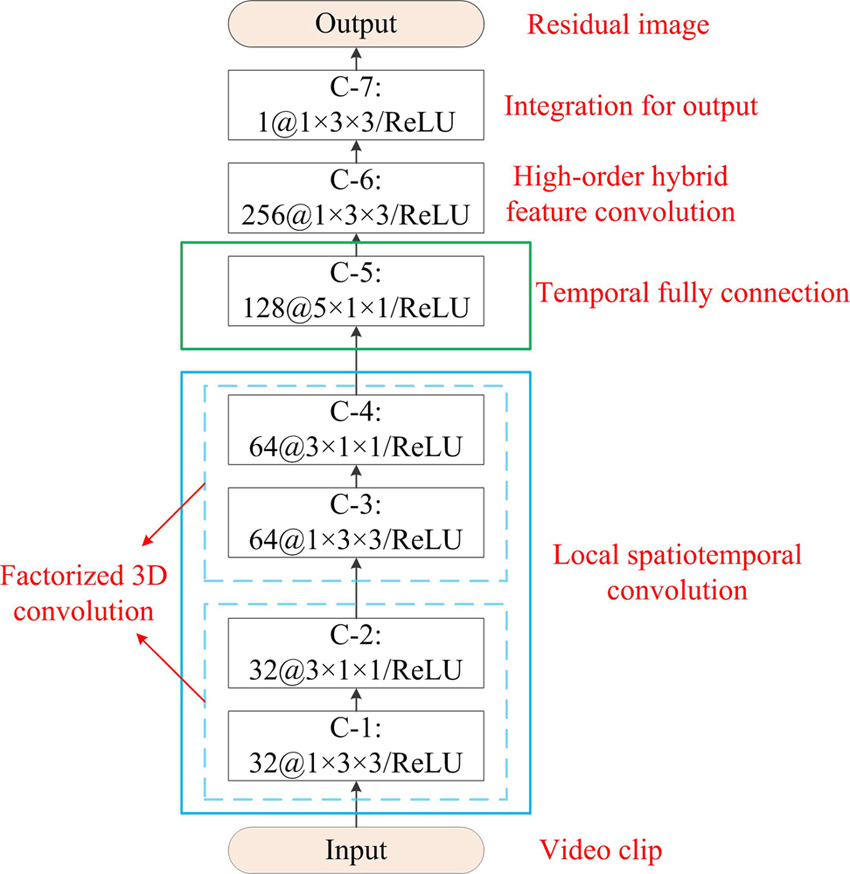
    Fig. 1. The proposed network architecture.
    The sketches of 3D covolution and factorized 3D convolution: (a) 3D covolution; (b) factorized 3D convolution.
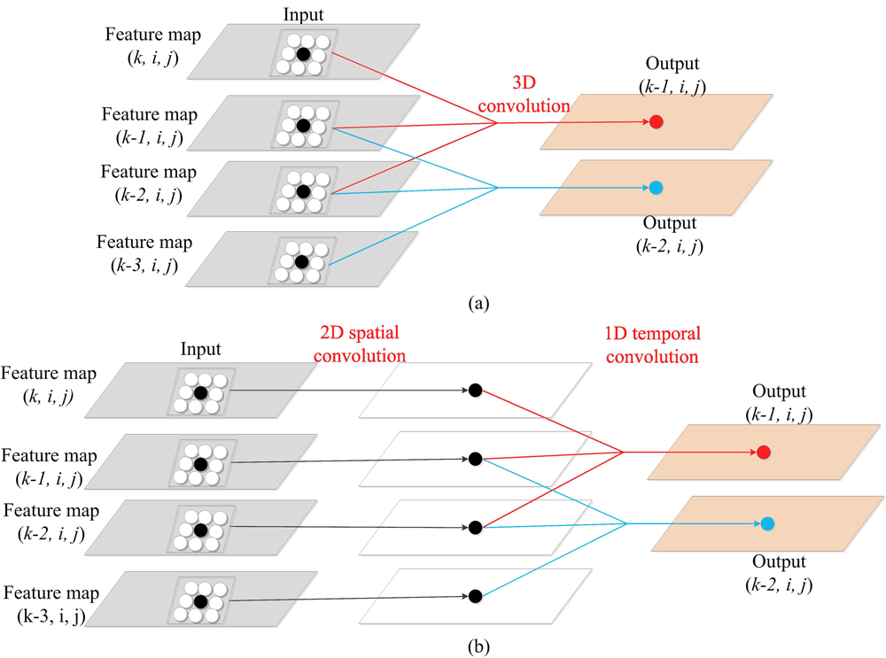
    Fig. 2. The sketches of 3D covolution and factorized 3D convolution: (a) 3D covolution; (b) factorized 3D convolution.
    The example of different error distributions: (a) the ground truth; (b) 1th predicted result with uniform error; (c) 2th predicted result with concentrated error.
    Fig. 3. The example of different error distributions: (a) the ground truth; (b) 1th predicted result with uniform error; (c) 2th predicted result with concentrated error.
    The function of intensity weighting parameter.
    Fig. 4. The function of intensity weighting parameter.
    The example of samples: (a) the target samples; (b) the background samples.
    Fig. 5. The example of samples: (a) the target samples; (b) the background samples.
    The original image and results of different methods for 1th Background.: (a) the original input; (b) the result of our method; (c) the result of Lin’s method; (d) the result of Max-Mean; (e) the result of TopHat; (f) the result of STDA.
    Fig. 6. The original image and results of different methods for 1th Background.: (a) the original input; (b) the result of our method; (c) the result of Lin’s method; (d) the result of Max-Mean; (e) the result of TopHat; (f) the result of STDA.
    The original image and results of different methods for 2th Background.: (a) the original input; (b) the result of our method; (c) the result of Lin’s method; (d) the result of Max-Mean; (e) the result of TopHat; (f) the result of STDA.
    Fig. 7. The original image and results of different methods for 2th Background.: (a) the original input; (b) the result of our method; (c) the result of Lin’s method; (d) the result of Max-Mean; (e) the result of TopHat; (f) the result of STDA.
    The original image and results of different methods for Target 1: (a) the original input; (b) the result of our method; (c) the result of Lin’s method; (d) the result of Max-Mean; (e) the result of TopHat; (f) the result of STDA.
    Fig. 8. The original image and results of different methods for Target 1: (a) the original input; (b) the result of our method; (c) the result of Lin’s method; (d) the result of Max-Mean; (e) the result of TopHat; (f) the result of STDA.
    The original image and results of different methods for Target 2: (a) the original input; (b) the result of our method; (c) the result of Lin’s method; (d) the result of Max-Mean; (e) the result of TopHat; (f) the result of STDA.
    Fig. 9. The original image and results of different methods for Target 2: (a) the original input; (b) the result of our method; (c) the result of Lin’s method; (d) the result of Max-Mean; (e) the result of TopHat; (f) the result of STDA.
    The display of Target 2: (a) the original gray image; (b) the standard deviation in the time domain.
    Fig. 10. The display of Target 2: (a) the original gray image; (b) the standard deviation in the time domain.
    The ROC curves of different methods.
    Fig. 11. The ROC curves of different methods.
    The result of different input size: (a) the input image with 35×35 pixels; (b) the result of image with35×35 pixels; (c) the input image with 45×45 pixels; (b) the result of image with45×45 pixels.
    Fig. 12. The result of different input size: (a) the input image with 35×35 pixels; (b) the result of image with35×35 pixels; (c) the input image with 45×45 pixels; (b) the result of image with45×45 pixels.
    The ROC curves with different jitters.
    Fig. 13. The ROC curves with different jitters.
    The ROC curves with different mean original SCRs.
    Fig. 14. The ROC curves with different mean original SCRs.
    ItemFlops(G)Parameters(K)
    3D Conv.0.0628.67
    Factorized 3D Conv.0.039.38
    Table 1. Computation comparison of different convolutions.
    ItemParameter
    CPUIntel i7,2.8GHz×12
    GPUNvidia-1080Ti
    RAM64GB
    SystemUbuntu 18.04
    Disk2TB
    SoftwarePytorch 1.1
    LanguagePython 3.6
    Table 2. The simulation environment.
    ProposedLin’sMax-MeanTopHatSTDA
    Target 120.406116.825320.930820.039419..8378
    Target 219.095311.92283.44103.062316.5872
    Mean19.750714.374112.185911.550918.2125
    Table 3. Background suppression comparison by SCR in output.
    ProposedLin’sMax-MeanTopHatSTAD
    Target 11.35271.02931.24771.12101.3375
    Target 27.18154.32181.25201.04315.5936
    Mean4.26712.67551.24981.08213.4656
    Table 4. Background suppression comparison by BSF.
    ProposedLin’sMax-MeanTopHatSTDA

    Average

    runtime(s)/sample

    5.84×10-43.38×10-43.30×10-31.33×10-24.51×10⁻³
    Table 5. Average runtime comparison.
    Miao LI, Zai-Ping LIN, Jian-Peng FAN, Wei-Dong SHENG, Jun LI, Wei AN, Xin-Lei LI. Point target detection based on deep spatial-temporal convolution neural network[J]. Journal of Infrared and Millimeter Waves, 2021, 40(1): 122
    Download Citation