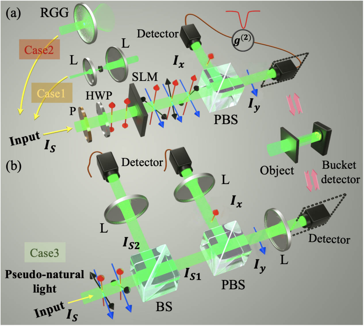
Fig. 1. (a) Schematic diagram of the PBS model: two CMOS-based image sensors (detectors) for recording intensity correlation. When the detector in the black-dotted box is replaced with an object and a bucket detector, the setup can facilitate GI experiments. A programmable SLM is utilized to generate the PF of the wavefront with adjustable coherence time. A 4-f lens system (not shown) is used to image the SLM plane onto the detection plane. (b) Schematic diagram of GI for pseudo-natural light: an ordinary BS is introduced to obtain additional reference beam for division and subtraction operations. P, linear polarizer; HWP, half-wave plate; L, lens; RGG, rotating ground glass.

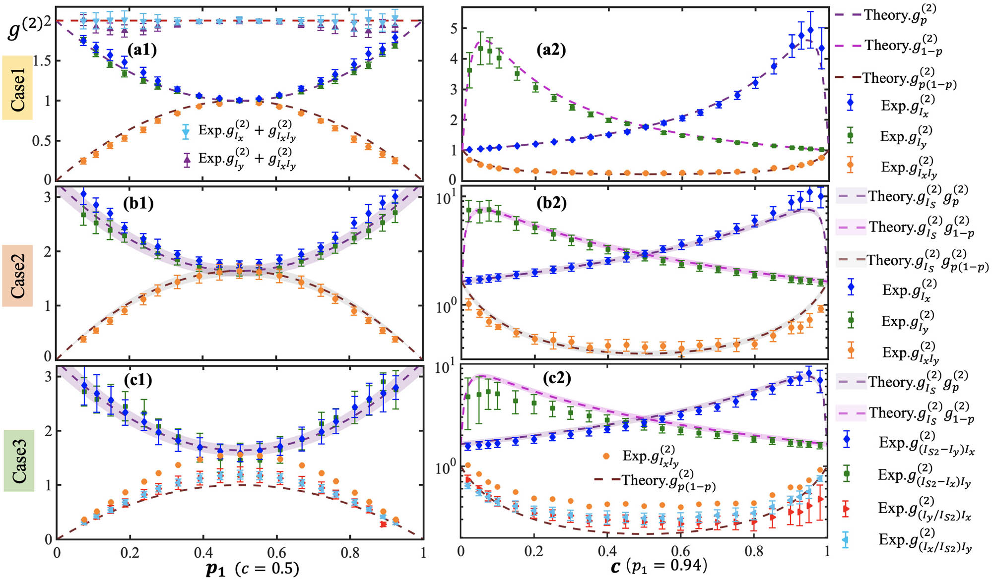
Fig. 2. Second-order correlation coefficients as functions of p1 and c for the symmetric Bernoulli distribution of PF. Case 1, coherent light with PF. (a1) Antibunching and bunching effects are exhibited in cross- and autocorrelation coefficients satisfying gp(2)+gp(1−p)(2)≈2; (a2) superbunching and antibunching effects can be observed with some values of c. Case 2 and Case 3, pseudo-thermal light with PF. (b1) and (b2) With the introduction of a statistically independent IF source, i.e., pseudo-thermal light, all the second-order correlation coefficients are multiplied by the second-order correlation coefficients of gIS(2), such that the superbunching is enhanced but the antibunching is weakened or even disappears. As a result, the cross-correlation coefficient of pseudo-thermal light is neither too high nor too low. To overcome this obstacle, division and subtraction are performed to gain anticorrelation and supercorrelation in (c1) and (c2) according to setup of Fig. 1(b). Note that (a1), (b1), and (c1) share the same abscissa with c fixed as 0.5, while (a2), (b2), and (c2) share the same abscissa with p1 fixed as 0.94. Also see the experimental calibration of the SLM in Appendix A.1.

Fig. 3. HBT curves of bunching and antibunching effects and corresponding GIs for different fluctuation sources. (a1) and (b1) Symmetric Bernoulli distribution of PF (p1=0.94, c=0.5); (a2) and (b2) uniform distribution of PF; (c1) and (d1) linearly polarized pseudo-thermal light of IF; (c2)–(c4) and (d2)–(d4) pseudo-natural light with both IF and PF (uniform distribution), where, in (c3) and (d3) division is performed, and in (c4) and (d4) subtraction is performed. 3000 shots contribute to each image, and scale bar is 1 mm, similarly hereinafter.

Fig. 4. Same as Fig. 3. The sources are pseudo-natural light with both IF and PF (symmetric Bernoulli distribution), where, in (a1) and (b1) p1=0.94, c=0.94, subtraction is performed; in (a2) and (b2) p1=0.94, c=0.5, division is performed.

Fig. 5. (a) Schematic diagram of GI with polarization identification. (b1) Positive image with IA only; (b2) negative image with IB only; (b3) polarization-sensitive image with both IA and IB. See Appendix A.3 for more experimental details.

Fig. 6. Schematic diagram of the customization of second-order correlation functions. Similar to Fig. 5, two independent fluctuation sources are combined. The difference is that an asymmetric offset is introduced in the PF path, which can be achieved by adjusting the angle of a mirror.

Fig. 7. Customization of various unique second-order correlation functions or point spread functions of the GI system. (a) Simulation object; (b1) hollow-like pattern; and (b2)–(b4) peak dip-like patterns with different directions by changing the angle of the mirror in Fig. 6. Note that only the middle area (96×96 pixels) is displayed in (b1)–(b4), where green lines are 1D distributions with the directions indicated by corresponding green arrows. (c1)–(c4) Simulation imaging results corresponding to different point spread functions; 500,000 shots contribute to each image. (d1)–(d4) Corresponding 1D profiles of images with the directions indicated by corresponding green arrows. The horizontal and longitudinal coordinates in (d1)–(d4) are pixel position and normalized intensity, respectively. For comparison, the solid line and the dashed line represent the edge-enhanced image and the original one, respectively.

Fig. 8. Experimental calibration of SLM. (a) Relationship between the parameter k loaded on the SLM and the light intensity of Ix, Iy, and IS (IS=Ix+Iy) using two photodetectors. The green translucent region in (b) can be approximately regarded as a symmetrical region (k ranges from 0.34 to 1 while p varies from 0.06 to 0.94, approximately).

Fig. 9. Raw measurement data of 800 shots that obey the Bernoulli distribution in the second-order correlation coefficient measurement.

Fig. 10. Raw speckle patterns of pseudo-thermal light. (a) Without and (b) with passing through the SLM.

Fig. 11. Probability density distributions of speckles for pseudo-natural light. (a) Spatial domain, statistics are made for all the speckles in a pattern of 600×960 pixels; (b) temporal domain, statistics are made for a certain pixel with 30,000 shots. Two kinds of pseudo-natural light models with uniform distribution and Bernoulli distribution (p1=0.94, c=0.5) are discussed in comparison with standard Rayleigh statistics.

Fig. 12. Experimental details of polarization-sensitive GI. (a) Experimental setup of second-order correlation coefficient measurement of the hybrid illumination and the polarization-sensitive GI. P, polarizer; R, reflector; ND, neutral density filter; HWP, half-wave plate; L, imaging lens; OBJ, object; the three optical elements (HWP-PBS-HWP) in the purple dotted box can continuously adjust the intensity and set the polarization angle of the IF source to be oriented at 45°. (b) Tunable correlation of the hybrid illumination with the change of the relative intensity ratio q, and the curve is fitted according to Eq. (A1). The polarization-sensitive GI experiment in the primary experiment is conducted at the condition of g(2)≈1, which is highlighted with the red dashed box in (b).