Antibunching and superbunching photon correlations in pseudo-natural light

Zhiyuan Ye; Hai-Bo Wang; Jun Xiong; Kaige Wang

doi:10.1364/PRJ.446935

Abstract

Since Hanbury Brown and Twiss revealed the photon bunching effect of a thermal light source in 1956, almost all studies in correlation optics have been based on light’s intensity fluctuation, regardless of fact that the polarization fluctuation is a basic attribute of natural light. In this work, we uncover the veil of the polarization fluctuation and corresponding photon correlations by proposing a new light source model, termed pseudo-natural light, embodying both intensity and polarization fluctuations. Unexpectedly, the strong antibunching and superbunching effects can be simultaneously realized in such a new source, whose second-order correlation coefficient

g^{(2)}

can be continuously modulated across 1. For the symmetric Bernoulli distribution of the polarization fluctuation, particularly,

g^{(2)}

can be in principle from 0 to unlimitedly large. In pseudo-natural light, while the bunching effects of both intensity and polarization fluctuations enhance the bunching to superbunching photon correlation, the antibunching correlation of the polarization fluctuation can also be extracted through the procedure of division operation in the experiment. The antibunching effect and the combination with the bunching one will arouse new applications in quantum imaging. As heuristic examples, we carry out high-quality positive or negative ghost imaging, and devise high-efficiency polarization-sensitive and edge-enhanced imaging. This work, therefore, sheds light on the development of multiple and broad correlation functions for natural light.

1. INTRODUCTION

In 1956, Hanbury Brown and Twiss (HBT) [1,2] proposed an intensity interferometer to measure the angular diameter of a star. The star light as natural light obeys the photon statistics of a thermal light field, i.e., the bunching correlation for bosons, where the second-order correlation coefficient $g^{(2)}$ of the optical field follows $1 < g^{(2)} \leq 2$ . The photon bunching in intensity correlation affords the coherence information of remote star light in an HBT intensity interferometer. Since the beginning of this century, the bunching correlation in thermal light has had many applications in a nonlocal imaging technique, such as ghost imaging (GI), ghost interference, and subwavelength interference [3 –15]. Especially, the GI technique has made widespread attention and revolutionary progress in the past decade. In these applications, most experiments employ the pseudo-thermal light source [16], which has a similar statistical correlation to the true thermal light but possesses a very slow temporal response.

Due to the Pauli exclusive principle and Fermi–Dirac statistics, fermions in a thermal source can manifest antibunching effect with $0 \leq g^{(2)} < 1$ [17 –19]. Gan et al. [20] proposed a scheme of magnifying GI of an electron microscope and pointed out that quantum imaging with thermal fermions can construct dark patterns against a bright intensity background. The dark image (or negative image) by antibunching correlation may increase the visibility perfectly against the maximum visibility of one-third for the positive GI by the bunching correlation of thermal photons. As for photons, however, the antibunching phenomenon is usually regarded as a signature of nonclassical light [21 –23], such as the photon number state. This distinguishing feature highlights the quantum nature of fermions without classical analog. It is worth noting that the classical anticorrelation phenomena can occur between reflected and transmitted speckle patterns from opaque disordered media [24,25], but the antibunching effect is very weak. On the other hand, the photon superbunching effect is meant for $g^{(2)} > 2$ , and it can also improve the visibility and resolution of GI. This effect can be carried out by nonlinear interaction between light and atoms [26 –29]. Recently, some simple and practical superbunching schemes for classical light were reported and can be applied to GI in the temporal domain [30] or in the spatial domain [31,32], and notably, these effects in classical regimes can be well interpreted by means of the speckle’s non-Rayleigh statistics [33 –35] in either the temporal or spatial domain. Also, some schemes have been proposed to generate a $g^{(2)}$ -switchable light source in the temporal domain [36] or in the spatial domain from coherent to thermal [37], from subthermal to superthermal [38], and controllable superthermal [39].

In conventional optical imaging, the most popular light sources come from natural sunlight. When sunlight is applied to GI, the main obstacle is its fast temporal fluctuation in the face of present, relatively slower response detectors. Liu et al. [40] performed the first experiment with lensless GI with sunlight, taking a step toward the practical application of natural light in GI. Natural light might contain both intensity fluctuation (IF) and polarization fluctuation (PF) [41], and several interesting models for the generalized HBT effect [42 –46] with a random vector field have been proposed. To our knowledge, however, most studies in correlation optics and imaging applications are based on light’s IF regardless of PF. In this work, we propose a simple scheme to exploit both antibunching and superbunching effects for PF in classical light. For the symmetric Bernoulli distribution of PF in coherent light, the spectrum of $g^{(2)}$ can be considerably broad, from zero for antibunching and unlimitedly large for superbunching. Similar to pseudo-thermal light, we introduce a pseudo-natural light source in which polarized pseudo-thermal light passes through a liquid crystal spatial light modulator (SLM) [47,48] to acquire independent IF and PF with much slower coherence time in comparison with polarization time of natural light [49]. In the pseudo-natural light model, the positive correlations of the IF and PF can be enhanced with each other to supercorrelation. However, the anticorrelation of PF can be extracted from the mixed correlations of PF and IF. Using the pseudo-natural light source, we perform high-quality positive and negative GI and carry out other relevant applications in the experiments.

Sign up for Photonics Research TOC. Get the latest issue of Photonics Research delivered right to you！Sign up now

2. THEORY

Considering a polarized beam of intensity $I_{S}$ passing through a polarizing beam splitter (PBS), as shown in Fig. 1(a), the intensities of two outgoing beams are given by $I_{x} = p I_{S}$ and $I_{y} = (1 - p) I_{S}$ , where $p \in [0,1]$ is a parameter related to the polarization state of the input beam. When input beam has the PF, $p$ becomes a random variable. We first consider the case when the input intensity $I_{S}$ is fixed, such as a laser beam. Due to the PF of the input beam, the two outgoing beams from PBS have the IF with $g_{I_{x}}^{(2)} = g_{p}^{(2)} = 1 + σ_{p}^{2} / μ_{p}^{2}$ and $g_{I_{y}}^{(2)} = g_{1 - p}^{(2)} = 1 + σ_{p}^{2} / {(1 - μ_{p})}^{2}$ , where we define $g_{I}^{(2)} = ⟨ I^{2} ⟩ / {⟨ I ⟩}^{2} = 1 + σ_{I}^{2} / μ_{I}^{2}$ with the mean value $μ_{I} = ⟨ I ⟩$ and variance $σ_{I}^{2} = ⟨ I^{2} ⟩ - {⟨ I ⟩}^{2}$ for the random variable $I$ . However, the cross-correlation function between the two outgoing beams is given by $g_{I_{x} I_{y}}^{(2)} = \frac{⟨ I_{x} I_{y} ⟩}{⟨ I_{x} ⟩ ⟨ I_{y} ⟩} = g_{p (1 - p)}^{(2)} = 1 - \frac{σ_{p}^{2}}{μ_{p} (1 - μ_{p})} .$ (1)

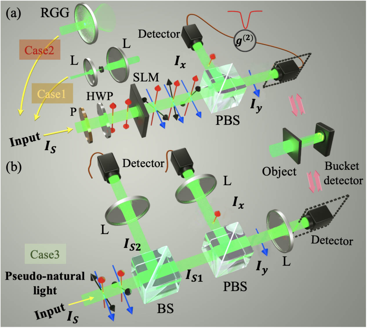
Figure 1.(a) Schematic diagram of the PBS model: two CMOS-based image sensors (detectors) for recording intensity correlation. When the detector in the black-dotted box is replaced with an object and a bucket detector, the setup can facilitate GI experiments. A programmable SLM is utilized to generate the PF of the wavefront with adjustable coherence time. A 4-f lens system (not shown) is used to image the SLM plane onto the detection plane. (b) Schematic diagram of GI for pseudo-natural light: an ordinary BS is introduced to obtain additional reference beam for division and subtraction operations. P, linear polarizer; HWP, half-wave plate; L, lens; RGG, rotating ground glass.

Since $0 \leq g_{p (1 - p)}^{(2)} < 1$ , the intensity-stable beam with the PF possesses the antibunching effect. When the horizontal and vertical polarization components balance out in the PF, i.e., $μ_{p} = 1 / 2$ , we get $g_{p}^{(2)} = g_{1 - p}^{(2)}$ and $g_{p}^{(2)} + g_{p (1 - p)}^{(2)} = 2$ .

To be clear, we show two examples. (i) Random linearly polarized light with polarization angle $θ$ , which is uniformly distributed in $[0, π]$ . We have $p = \cos^{2} θ$ , $μ_{p} = 1 / 2$ , $⟨ p^{2} ⟩ = 3 / 8$ , $σ_{p}^{2} = 1 / 8$ , and obtain $g_{p}^{(2)} = g_{1 - p}^{(2)} = 3 / 2$ and $g_{p (1 - p)}^{(2)} = 1 / 2$ . (ii) Linearly polarized light with only two polarization angles, i.e., a Bernoulli distribution. The probability function for random variable $p$ is $P (p) = {\begin{matrix} c, p = p_{1} \\ 1 - c, p = p_{2} \end{matrix}$ , where $0 < c < 1$ and $p_{1} \neq p_{2}$ . We can calculate $μ_{p} = p_{1} c + p_{2} (1 - c)$ , $⟨ p^{2} ⟩ = p_{1}^{2} c + p_{2}^{2} (1 - c)$ , $σ_{p}^{2} = c (1 - c) {(p_{1} - p_{2})}^{2}$ , and accordingly, $g_{p}^{(2)}$ , $g_{1 - p}^{(2)}$ , and $g_{p (1 - p)}^{(2)}$ . For example, in the symmetric configuration of $p_{1} + p_{2} = 1$ , we have $μ_{p} = p_{1} c + (1 - p_{1}) (1 - c)$ and $σ_{p}^{2} = c (1 - c) (2 p_{1} - {1)}^{2}$ . Especially if the beam contains only horizontal and vertical polarization states, we obtain $g_{p}^{(2)} = 1 / c$ , $g_{1 - p}^{(2)} = 1 / (1 - c)$ , and $g_{p (1 - p)}^{(2)} = 0$ . The minimum antibunching effect is realized, since in this case every photon chooses only one way in the PBS with certainty. However, the maximum superbunching effect ( $g_{p}^{(2)}$ or $g_{1 - p}^{(2)}$ ) can be unlimitedly large as $c$ is close to 0 or 1.

A general polarization state of monochromatic plane wave can be described by the Stokes vector on the Poincaré sphere [50], $\begin{array}{l} \begin{array}{l} (\begin{matrix} S_{0} \\ S_{1} \\ S_{2} \\ S_{3} \end{matrix}) = I_{S} (\begin{matrix} 1 \\ \cos (2 χ) \cos (2 ψ) \\ \cos (2 χ) \sin (2 ψ) \\ \sin (2 χ) \end{matrix}), \end{array} \end{array}$ (2)where $ψ$ ( $0 \leq ψ \leq π$ ) specifies the orientation and $χ$ ( $- π / 4 \leq χ \leq π / 4$ ) characterizes the ellipticity of the polarization ellipse, while $2 χ$ and $2 ψ$ stand for the spherical angular coordinates of latitude and longitude, respectively. When the intensity of a plane wave is given, $S_{0} = I_{S}$ ; thus, it has defined the radius of the Poincaré sphere. The probability function $P (2 χ,2 ψ)$ on the Poincaré sphere can describe the PF. Because of $S_{1} = I_{x} - I_{y} = (2 p - 1) I_{S}$ , it has $p = (\cos 2 χ \cos 2 ψ + 1) / 2$ . As a result, we can calculate $⟨ p ⟩$ , $⟨ p^{2} ⟩$ on the Poincaré sphere, and the corresponding second-order correlation functions. For example, for the uniform probability distribution on the Poincaré sphere $P (2 χ, 2 ψ) = 1 / 4 π$ , we have $μ_{p} = 1 / 2$ , $σ_{p}^{2} = 1 / 12$ , $g_{p}^{(2)} = g_{1 - p}^{(2)} = 4 / 3$ , and $g_{p (1 - p)}^{(2)} = 2 / 3$ . Both bunching and antibunching effects coexist, and $g_{p}^{(2)} + g_{p (1 - p)}^{(2)} = 2$ . As for the case of random circularly polarized light, which has only left-handed and right-handed states (the north pole and south pole on the Poincaré sphere), the IF will not exist after passing through a PBS. To gain the IF, however, one can introduce a quarter-wave plate in front of the PBS.

We now consider the case in which the beam of intensity $I_{S}$ contains both IF and PF, which are independent of each other, possibly similar to some of natural light. When the beam impinges on a PBS, three second-order correlation coefficients of two outgoing beams are obtained to be $g_{I_{x}}^{(2)} = g_{I_{S}}^{(2)} g_{p}^{(2)}, g_{I_{y}}^{(2)} = g_{I_{S}}^{(2)} g_{1 - p}^{(2)}, g_{I_{x} I_{y}}^{(2)} = g_{I_{S}}^{(2)} g_{p (1 - p)}^{(2)} .$ (3)

The intensity correlation functions of outgoing beams from the PBS can be factorized according to independent IF and PF. Since $g_{I_{S}}^{(2)}$ , $g_{p}^{(2)}$ , and $g_{1 - p}^{(2)}$ are positive correlation functions ( $g^{(2)} > 1$ ), $g_{I_{x}}^{(2)}$ and $g_{I_{y}}^{(2)}$ are also positive correlation ones, possibly superbunching. However, $g_{p (1 - p)}^{(2)}$ is an anticorrelation one ( $g^{(2)} < 1$ ), so the cross-intensity correlation $g_{I_{x} I_{y}}^{(2)}$ may be positive or anticorrelation, depending on the competition between two opposite correlations. Hence, in the PBS scheme, the IF of the input beam enhances the positive correlation of each polarization mode while counteracting the anticorrelation between two polarization modes. It would be an obstacle to gain the antibunching effect for natural light.

To surpass the obstacle, we propose a scheme of combination of a beam splitter (BS) and a PBS in Fig. 1(b). The pseudo-natural light is divided into two parts after the BS with the intensities $I_{S 1} = t I_{S}$ and $I_{S 2} = r I_{S}$ , where $t$ and $r$ are the transmissivity and the reflectivity of the BS, respectively. After the PBS, the intensities of the two outgoing beams for the horizontal and vertical polarization modes are written as $I_{x} = p I_{S 1} = p t I_{S}$ and $I_{y} = (1 - p) I_{S 1} = (1 - p) t I_{S}$ . It is clear that the second-order correlation functions of $I_{x}$ and $I_{y}$ follow Eq. (3) because of $g_{I_{S 1}}^{(2)} = g_{I_{S}}^{(2)}$ .

We now perform some basic operations between the random variables $I_{S 2}$ and $I_{x}$ ( $I_{y}$ ). First, we define the division operations $p_{x} \equiv I_{x} / I_{S 2} = (t / r) p$ and $p_{y} \equiv I_{y} / I_{S 2} = (t / r) (1 - p)$ , so the random intensity of the carrier beam has been eliminated. Thus we obtain $g_{p_{x} I_{x}}^{(2)} = g_{p_{x}}^{(2)} = g_{p}^{(2)}, g_{p_{y} I_{y}}^{(2)} = g_{p_{y}}^{(2)} = g_{1 - p}^{(2)}, g_{p_{x} I_{y}}^{(2)} = g_{I_{x} p_{y}}^{(2)} = g_{p_{x} p_{y}}^{(2)} = g_{p (1 - p)}^{(2)} .$ (4)

As a result, all the correlation functions related to the PF only have been extracted. Second, we introduce the subtraction operations $I_{S 2} - I_{x} = (r - p t) I_{S}$ and $I_{S 2} - I_{y} = [r - (1 - p) t] I_{S}$ , and calculate the cross-correlation functions, $g_{(I_{S 2} - I_{x}) I_{y}}^{(2)} = \frac{(1 - 2 t) (1 - ⟨ p ⟩) + t ⟨ {(1 - p)}^{2} ⟩}{(1 - 2 t) (1 - ⟨ p ⟩) + t {⟨ (1 - p) ⟩}^{2}} g_{I_{S}}^{(2)}, g_{(I_{S 2} - I_{y}) I_{x}}^{(2)} = \frac{(1 - 2 t) ⟨ p ⟩ + t ⟨ p^{2} ⟩}{(1 - 2 t) ⟨ p ⟩ + t {⟨ p ⟩}^{2}} g_{I_{S}}^{(2)},$ (5)where the lossless BS condition $r + t = 1$ has been applied. For a balanced lossless BS, we arrive at $g_{(I_{S 2} - I_{x}) I_{y}}^{(2)} = g_{1 - p}^{(2)} g_{I_{S}}^{(2)}, g_{(I_{S 2} - I_{y}) I_{x}}^{(2)} = g_{p}^{(2)} g_{I_{S}}^{(2)} .$ (6)

The results are exactly the same as the first two equations in Eq. (3), but here the cross-correlations of two polarization modes replace the autocorrelations of each polarization mode. Since two correlated beams are ready, the present method is convenient for GI performance.

3. RESULTS

A. Experimental Observations of Antibunching and Superbunching

In the experimental performance, we discuss three cases for the PF of the Bernoulli distribution with the symmetrical polarization configuration $p_{1} + p_{2} = 1$ (see the experimental calibration of the SLM in Appendix A.1). In Case 1 and Case 2, coherent light and pseudo-thermal light drive the SLM, respectively; then these beams are injected onto a PBS, shown in Fig. 1(a). In Case 3, however, pseudo-thermal light drives the SLM to form pseudo-natural light with independent IF and PF as Case 2; then pseudo-natural light impinges on a BS and follows the PBS, shown in Fig. 1(b). We measure the second-order correlation coefficients as functions of $p_{1}$ and $c$ in Fig. 2.

Figure 2.Second-order correlation coefficients as functions of $p_{1}$ and $c$ for the symmetric Bernoulli distribution of PF. Case 1, coherent light with PF. (a1) Antibunching and bunching effects are exhibited in cross- and autocorrelation coefficients satisfying $g_{p}^{(2)} + g_{p (1 - p)}^{(2)} \approx 2$ ; (a2) superbunching and antibunching effects can be observed with some values of $c$ . Case 2 and Case 3, pseudo-thermal light with PF. (b1) and (b2) With the introduction of a statistically independent IF source, i.e., pseudo-thermal light, all the second-order correlation coefficients are multiplied by the second-order correlation coefficients of $g_{I_{S}}^{(2)}$ , such that the superbunching is enhanced but the antibunching is weakened or even disappears. As a result, the cross-correlation coefficient of pseudo-thermal light is neither too high nor too low. To overcome this obstacle, division and subtraction are performed to gain anticorrelation and supercorrelation in (c1) and (c2) according to setup of Fig. 1(b). Note that (a1), (b1), and (c1) share the same abscissa with $c$ fixed as 0.5, while (a2), (b2), and (c2) share the same abscissa with $p_{1}$ fixed as 0.94. Also see the experimental calibration of the SLM in Appendix A.1.

For Case 1, when the coherent light drives the SLM, we can observe $g_{p}^{(2)}$ , $g_{1 - p}^{(2)}$ , and $g_{p (1 - p)}^{(2)}$ of PF directly in Figs. 2(a1) and 2(a2). In Fig. 2(a1) [also Figs. 2(b1) and 2(c1)], the probability of two polarization modes is balanced as $c = 1 / 2$ . The experimental results demonstrate the positive correlation $g_{p}^{(2)} = g_{1 - p}^{(2)} > 1$ and anticorrelation $g_{p (1 - p)}^{(2)} < 1$ (from 0.25 to 0.99), approximately satisfying $g_{p}^{(2)} + g_{p (1 - p)}^{(2)} = 2$ . In Fig. 2(a2) [also Figs. 2(b2) and 2(c2)], the maximum linear polarization parameter $p_{1} = 0.94$ in the SLM is taken; then we have the minimum anticorrelation $g_{p (1 - p)}^{(2)} = 0.25 \pm 0.03$ at $c = 1 / 2$ . However, larger positive correlation coefficients (superbunching effect) for each outgoing polarization mode $g_{p}^{(2)} = 5 \pm 0.6$ and $g_{1 - p}^{(2)} = 4.3 \pm 0.5$ are generated for $c = 0.94$ and 0.06, respectively.

For Case 2 we measure $g_{I_{x}}^{(2)}$ , $g_{I_{y}}^{(2)}$ , and $g_{I_{x} I_{y}}^{(2)}$ for pseudo-natural light in Figs. 2(b1) and 2(b2). These second-order correlation coefficients are similar to $g_{p}^{(2)}$ , $g_{1 - p}^{(2)}$ , and $g_{p (1 - p)}^{(2)}$ in Figs. 2(a1) and 2(a2) but enhanced by $g_{I_{S}}^{(2)} = 1.6 \pm 0.1$ due to Eq. (3). As a result, the enhanced superbunching effect can be observed with the maximum values of 10.3 and 8.1 at $c = 0.94$ and 0.06, respectively. However, the cross-correlation coefficient $g_{I_{x} I_{y}}^{(2)}$ varies from 0.38 to 1.64 in Fig. 2(b1), i.e., from anticorrelation to positive correlation, against the whole anticorrelation in Case 1.

For Case 3, by combination of an ordinary BS and a PBS in Fig. 1(b), we perform the division operation and subtraction operation mentioned above to obtain the original antibunching correlation of PF and superbunching correlation of both IF and PF, respectively. By the division operation, $g_{p_{x} I_{y}}^{(2)}$ and $g_{I_{x} p_{y}}^{(2)}$ are measured in the range of 0.31–1.21 with respect to the range of 0.38–1.64 for $g_{I_{x} I_{y}}^{(2)}$ [see lower part in Fig. 2(c1)]. Since very small intensities will give incorrect results, these records have to be deleted in the division. For this reason, the IF is partly eliminated. As seen in Fig. 2(c2), by the subtraction operation the superbunching effect can be realized with the maximum records of 8.3 and 6.0 at $c = 0.94$ and 0.08, respectively.

In the experiment, the values of p are limited by the SLM and PBS in the range $[0.06, 0.94]$ (see Appendix A.1 for the experimental calibration of the SLM and error analysis). So, we can observe the second-order correlation coefficients ranging from a minimum of 0.25 to a maximum of 10.3. Hence, this simple setup can be viewed as a special light source with tunable photon correlation from antibunching to superbunching.

B. Positive and Negative Ghost Images

Next, we observe HBT curves and perform GI experiments. As shown in Fig. 1, the detector in the dotted box is replaced with an object and a bucket detector. The experimental results are presented in Figs. 3 and 4. We first consider the PF source driven by coherent light. For the symmetric Bernoulli distribution ( $p_{1} = 0.94$ , $c = 0.5$ ) and uniform distribution of PF, the antibunching HBT curves with the minimum $g_{I_{x} I_{y}}^{(2)} = 0.26$ and 0.54 are plotted in Figs. 3(a1) and 3(a2), respectively. As a result, we observe dark ghost images in Figs. 3(b1) and 3(b2) with much better contrast-to-noise ratio (CNR, also see Eqs. (A2) and (A3) in Appendix A.4) [51].

Figure 3.HBT curves of bunching and antibunching effects and corresponding GIs for different fluctuation sources. (a1) and (b1) Symmetric Bernoulli distribution of PF ( $p_{1} = 0.94$ , $c = 0.5$ ); (a2) and (b2) uniform distribution of PF; (c1) and (d1) linearly polarized pseudo-thermal light of IF; (c2)–(c4) and (d2)–(d4) pseudo-natural light with both IF and PF (uniform distribution), where, in (c3) and (d3) division is performed, and in (c4) and (d4) subtraction is performed. 3000 shots contribute to each image, and scale bar is 1 mm, similarly hereinafter.

Figure 4.Same as Fig. 3. The sources are pseudo-natural light with both IF and PF (symmetric Bernoulli distribution), where, in (a1) and (b1) $p_{1} = 0.94$ , $c = 0.94$ , subtraction is performed; in (a2) and (b2) $p_{1} = 0.94$ , $c = 0.5$ , division is performed.

In Fig. 4, pseudo-natural light is formed with the symmetric Bernoulli distribution of PF driven by pseudo-thermal light. We consider two cases: ( $p_{1} = 0.94$ , $c = 0.94$ ) in Figs. 4(a1) and 4(b1) and ( $p_{1} = 0.94$ , $c = 0.5$ ) in Figs. 4(a2) and 4(b2). For the former, we perform the subtraction operation and observe the significant superbunching effect ( $g^{(2)} = 8.43$ ). As for the latter, we perform the division operation and extract the antibunching effect of PF ( $g^{(2)} = 0.32$ ). Hence the corresponding positive image in Fig. 4(b1) and negative image in Fig. 4(b2) have much better CNRs.

C. Polarization-Sensitive GI

The combination of two opposite photon correlations can find a variety of applications. Here we demonstrate polarization-sensitive imaging as getting started, which is developed to enhance the visibility of targets in scattering media [52]. As shown in Fig. 5(a), $I_{A}$ and $I_{B}$ are intensities of two independent light sources A and B with IF and PF, respectively. Beam A is linearly polarized with a solid angle oriented at 45°. Two beams are mixed in a PBS to generate a hybrid illumination. The targets are now polarized—two letters have orthogonal polarization. When source B (A) is turned off, the positive (negative) image appears for the horizontally (vertically) polarized letter, as shown in Fig. 5(b1) [Fig. 5(b2)], which is also illustrated by the inset table in Fig. 5(a). For the hybrid illumination, however, two letters appear simultaneously and identifiably in Fig. 5(b3) with diametrically opposite intensity below and above the background. This feature is superior to the common scheme of polarization-sensitive imaging. Also see Appendix A.3 for more experimental details. It is worth noting that the present scheme can achieve resolution-enhanced measurement of polarization-sensitive phase objects, just like the recent work on polarization entanglement-enabled quantum holography, proposed by Defienne et al. [53].

Figure 5.(a) Schematic diagram of GI with polarization identification. (b1) Positive image with $I_{A}$ only; (b2) negative image with $I_{B}$ only; (b3) polarization-sensitive image with both $I_{A}$ and $I_{B}$ . See Appendix A.3 for more experimental details.

D. Customization of the Spatial Pattern of Second-Order Correlation Functions

In general, the combination of classical spatial antibunching and bunching effects also provides an alternative toolbox for the customization of the second-order correlation functions. For example, the second-order correlation coefficient can be continuously adjustable in a wide range across 1, which has been shown in Fig. 2. Also, the spatial structure of the second-order correlation function can be tailored based on the opposite spatial correlation distributions.

The schematic diagram of the second example is shown in Fig. 6, which is very similar to Fig. 5(a), but the two beams corresponding to independent IF and PF sources are offset by an adjustable mirror. Figure 7(a) shows the simulation object ( $256 \times 256$ pixels). The size of the speckle unit, i.e., the half-height width of the second-order correlation function, is set to $\sim 6$ pixels. First, we introduce the customization of a hollow-like pattern of the second-order correlation function shown in Fig. 7(b1): no offset, but the size of the speckle unit of the IF source is increased to $\sim 9$ pixels. As a result, the central area of the second-order correlation function is about 1, while the surrounding region is larger than 1, and a fuzzy positive image is shown in Fig. 7(c1).

Figure 6.Schematic diagram of the customization of second-order correlation functions. Similar to Fig. 5, two independent fluctuation sources are combined. The difference is that an asymmetric offset is introduced in the PF path, which can be achieved by adjusting the angle of a mirror.

Figure 7.Customization of various unique second-order correlation functions or point spread functions of the GI system. (a) Simulation object; (b1) hollow-like pattern; and (b2)–(b4) peak dip-like patterns with different directions by changing the angle of the mirror in Fig. 6. Note that only the middle area ( $96 \times 96$ pixels) is displayed in (b1)–(b4), where green lines are 1D distributions with the directions indicated by corresponding green arrows. (c1)–(c4) Simulation imaging results corresponding to different point spread functions; 500,000 shots contribute to each image. (d1)–(d4) Corresponding 1D profiles of images with the directions indicated by corresponding green arrows. The horizontal and longitudinal coordinates in (d1)–(d4) are pixel position and normalized intensity, respectively. For comparison, the solid line and the dashed line represent the edge-enhanced image and the original one, respectively.

Then we introduce the offset of six pixels between the two beams. Two spots with a peak and a dip in the second-order correlation functions are formed with different directions [Figs. 7(b2)–7(b4)] by adjusting the angle of the mirror. With these tailored second-order correlation functions, we can observe the various reconstructed images [Figs. 7(c2)–7(c4)] with edges enhanced at corresponding directions. For comparisons of edge quality, Figs. 7(d1)–7(d4) show one-dimensional (1D) profiles of images in the direction of the corresponding arrow. Hence, the introduction of PF has expanded more unexpected possibilities for GI applications.

4. CONCLUSION

In summary, we have demonstrated antibunching and superbunching effects in the PF of classical light and applied them to high-quality positive and negative GI, and proposed two application examples. Usually either the superbunching effect or the anti-bunching effect can be found in some quantum optical systems. Our model is completely limited in the scope of classical optics but covers both superbunching and antibunching effects. The present scheme is very simple and significantly effective for a special light source with a multiple and broad correlation property. At present, however, while pseudo-thermal light with IF only is still the most popular source in correlation optics, our work affords an alternative choice with enhancements. Sunlight offers humans a visible world free of charge. As natural sunlight contains both IF and PF, our work also opens the way for wide applications for natural light.

APPENDIX A

1.Experimental Calibration of the SLM

\sim 64 %

Figure 8.Experimental calibration of SLM. (a) Relationship between the parameter $k$ loaded on the SLM and the light intensity of $I_{x}$ , $I_{y}$ , and $I_{S}$ ( $I_{S} = I_{x} + I_{y}$ ) using two photodetectors. The green translucent region in (b) can be approximately regarded as a symmetrical region ( $k$ ranges from 0.34 to 1 while $p$ varies from 0.06 to 0.94, approximately).

Figure 9.Raw measurement data of 800 shots that obey the Bernoulli distribution in the second-order correlation coefficient measurement.

Figure 10.Raw speckle patterns of pseudo-thermal light. (a) Without and (b) with passing through the SLM.

Figure 11.Probability density distributions of speckles for pseudo-natural light. (a) Spatial domain, statistics are made for all the speckles in a pattern of $600 \times 960$ pixels; (b) temporal domain, statistics are made for a certain pixel with 30,000 shots. Two kinds of pseudo-natural light models with uniform distribution and Bernoulli distribution ( $p_{1} = 0.94$ , $c = 0.5$ ) are discussed in comparison with standard Rayleigh statistics.

Figure 12.Experimental details of polarization-sensitive GI. (a) Experimental setup of second-order correlation coefficient measurement of the hybrid illumination and the polarization-sensitive GI. P, polarizer; R, reflector; ND, neutral density filter; HWP, half-wave plate; L, imaging lens; OBJ, object; the three optical elements (HWP-PBS-HWP) in the purple dotted box can continuously adjust the intensity and set the polarization angle of the IF source to be oriented at 45°. (b) Tunable correlation of the hybrid illumination with the change of the relative intensity ratio $q$ , and the curve is fitted according to Eq. (A1). The polarization-sensitive GI experiment in the primary experiment is conducted at the condition of $g^{(2)} \approx 1$ , which is highlighted with the red dashed box in (b).

In almost all imaging modalities, to obtain a polarization-sensitive image, one must collect the two images of two mutually orthogonal components, and then complete the differential operation in the postprocessing. However, in our GI modality, by multiplexing bunching and antibunching into two orthogonal polarization components, only a single round of acquisition is required, and no subsequent differential operations are needed. It is an interesting and special feature that only occurs in GI modality using the hybrid illumination. Also, the edge-enhanced GI experiment presented in Fig. 7 has similar advantages.

4.Definition of CNR

G (x)

References

[1] R. H. Brown, R. Q. Twiss. Correlation between photons in two coherent beams of light. Nature, 177, 27-29(1956).

[2] R. H. Brown, R. Q. Twiss. A test of a new type of stellar interferometer on Sirius. Nature, 178, 1046-1048(1956).

[3] R. S. Bennink, S. J. Bentley, R. W. Boyd. Two-photon’ coincidence imaging with a classical source. Phys. Rev. Lett., 89, 113601(2002).

[4] R. S. Bennink, S. J. Bentley, R. W. Boyd, J. C. Howell. Quantum and classical coincidence imaging. Phys. Rev. Lett., 92, 033601(2004).

[5] A. Gatti, E. Brambilla, M. Bache, L. A. Lugiato. Ghost imaging with thermal light: comparing entanglement and classical correlation. Phys. Rev. Lett., 93, 093602(2004).

[6] Y. Cai, S. Y. Zhu. Ghost interference with partially coherent radiation. Opt. Lett., 29, 2716-2718(2004).

[7] K. Wang, D. Z. Cao. Subwavelength coincidence interference with classical thermal light. Phys. Rev. A, 70, 041801(2004).

[8] J. Cheng, S. Han. Incoherent coincidence imaging and its applicability in X-ray diffraction. Phys. Rev. Lett., 92, 093903(2004).

[9] D. Z. Cao, J. Xiong, K. Wang. Geometrical optics in correlated imaging systems. Phys. Rev. A, 71, 013801(2005).

[10] F. Ferri, D. Magatti, A. Gatti, M. Bache, E. Brambilla, L. A. Lugiato. High-resolution ghost image and ghost diffraction experiments with thermal light. Phys. Rev. Lett., 94, 183602(2005).

[11] A. Valencia, G. Scarcelli, M. D’Angelo, Y. Shih. Two-photon imaging with thermal light. Phys. Rev. Lett., 94, 063601(2005).

[12] J. Xiong, D. Z. Cao, F. Huang, H. G. Li, X. J. Sun, K. Wang. Experimental observation of classical subwavelength interference with a pseudothermal light source. Phys. Rev. Lett., 94, 173601(2005).

[13] D. Zhang, Y. H. Zhai, L. A. Wu, X. H. Chen. Correlated two-photon imaging with true thermal light. Opt. Lett., 30, 2354-2356(2005).

[14] D. Z. Cao, J. Xiong, S. H. Zhang, L. F. Lin, L. Gao, K. Wang. Enhancing visibility and resolution in Nth-order intensity correlation of thermal light. Appl. Phys. Lett., 92, 201102(2008).

[15] J. H. Shapiro. Computational ghost imaging. Phys. Rev. A, 78, 061802(2008).

[16] F. T. Arecchi. Measurement of the statistical distribution of Gaussian and laser sources. Phys. Rev. Lett., 15, 912-916(1965).

[17] R. C. Liu, B. Odom, Y. Yamamoto, S. Tarucha. Quantum interference in electron collision. Nature, 391, 263-265(1998).

[18] M. Henny, S. Oberholzer, C. Strunk, T. Heinzel, K. Ensslin, M. Holland, C. Schönenberger. The fermionic Hanbury Brown and Twiss experiment. Science, 284, 296-298(1999).

[19] H. Kiesel, A. Renz, F. Hasselbach. Observation of Hanbury Brown-Twiss anticorrelations for free electrons. Nature, 418, 392-394(2002).

[20] S. Gan, D. Z. Cao, K. Wang. Dark quantum imaging with fermions. Phys. Rev. A, 80, 043809(2009).

[21] H. J. Kimble, M. Dagenais, L. Mandel. Photon antibunching in resonance fluorescence. Phys. Rev. Lett., 39, 691-695(1977).

[22] P. Michler, A. Imamoglu, M. D. Mason, P. J. Carson, G. F. Strouse, S. K. Buratto. Quantum correlation among photons from a single quantum dot at room temperature. Nature, 406, 968-970(2000).

[23] R. Boddeda, Q. Glorieux, A. Bramati, S. Pigeon. Generating strong anti-bunching by interfering nonclassical and classical states of light. J. Phys. B, 52, 215401(2019).

[24] I. Starshynov, A. M. Paniagua-Diaz, N. Fayard, A. Goetschy, R. Pierrat, R. Carminati, J. Bertolotti. Non-Gaussian correlations between reflected and transmitted intensity patterns emerging from opaque disordered media. Phys. Rev. X, 8, 021041(2018).

[25] A. M. Paniagua-Diaz, I. Starshynov, N. Fayard, A. Goetschy, R. Pierrat, R. Carminati, J. Bertolotti. Blind ghost imaging. Optica, 6, 460-464(2019).

[26] T. Grujic, S. R. Clark, D. Jaksch, D. G. Angelakis. Repulsively induced photon superbunching in driven resonator arrays. Phys. Rev. A, 87, 053846(2013).

[27] Z. Ficek. Highly directional photon superbunching from a few-atom chain of emitters. Phys. Rev. A, 98, 063824(2018).

[28] M. Marconi, J. Javaloyes, P. Hamel, F. Raineri, A. Levenson, A. M. Yacomotti. Far-from-equilibrium route to superthermal light in bimodal nanolasers. Phys. Rev. X, 8, 011013(2018).

[29] C. C. Leon, A. Rosławska, A. Grewal, O. Gunnarsson, K. Kuhnke, K. Kern. Photon superbunching from a generic tunnel junction. Sci. Adv., 5, eaav4986(2019).

[30] Y. Zhou, F. L. Li, B. Bai, H. Chen, J. Liu, Z. Xu, H. Zheng. Superbunching pseudothermal light. Phys. Rev. A, 95, 053809(2017).

[31] L. Zhang, Y. Lu, D. Zhou, H. Zhang, L. Li, G. Zhang. Superbunching effect of classical light with a digitally designed spatially phase-correlated wave front. Phys. Rev. A, 99, 063827(2019).

[32] F. Gori, M. Santarsiero. Spatial superbunching of light: model sources. Opt. Lett., 44, 4012-4015(2019).

[33] N. Bender, H. Yılmaz, Y. Bromberg, H. Cao. Creating and controlling complex light. APL Photonics, 4, 110806(2019).

[34] A. Roy, M. M. Brundavanam. Polarization-based intensity correlation of a depolarized speckle pattern. Opt. Lett., 46, 4896-4899(2021).

[35] C. Q. Wei, J. B. Liu, X. X. Zhang, R. Zhuang, Y. Zhou, H. Chen, Y. C. He, H. B. Zheng, Z. Xu. Non-Rayleigh photon statistics of superbunching pseudothermal light. Chin. Phys. B, 31, 024209(2022).

[36] I. Straka, J. Mika, M. Ježek. Generator of arbitrary classical photon statistics. Opt. Express, 26, 8998-9010(2018).

[37] M. Blazek, W. Elsäßer. Coherent and thermal light: tunable hybrid states with second-order coherence without first-order coherence. Phys. Rev. A, 84, 063840(2011).

[38] H. E. Kondakci, A. Szameit, A. F. Abouraddy, D. N. Christodoulides, B. E. A. Saleh. Sub-thermal to super-thermal light statistics from a disordered lattice via deterministic control of excitation symmetry. Optica, 3, 477-482(2016).

[39] S. Zhang, H. Zheng, G. Wang, J. Liu, S. Luo, Y. He, Y. Zhou, H. Chen, Z. Xu. Controllable superbunching effect from four-wave mixing process in atomic vapor. Opt. Express, 28, 21489-21498(2020).

[40] X. F. Liu, X. H. Chen, X. R. Yao, W. K. Yu, G. J. Zhai, L. A. Wu. Lensless ghost imaging with sunlight. Opt. Lett., 39, 2314-2317(2014).

[41] A. Shevchenko, T. Setälä, M. Kaivola, A. T. Friberg. Characterization of polarization fluctuations in random electromagnetic beams. New J. Phys., 11, 073004(2009).

[42] T. Shirai, E. Wolf. Correlations between intensity fluctuations in stochastic electromagnetic beams of any state of coherence and polarization. Opt. Commun., 272, 289-292(2007).

[43] X. Liu, G. Wu, X. Pang, D. Kuebel, T. D. Visser. Polarization and coherence in the Hanbury Brown-Twiss effect. J. Mod. Opt., 65, 1437-1441(2018).

[44] D. Kuebel, T. D. Visser. Generalized Hanbury Brown-Twiss effect for Stokes parameters. J. Opt. Soc. Am. A, 36, 362-367(2019).

[45] G. Wu, D. Kuebel, T. D. Visser. Generalized Hanbury Brown-Twiss effect in partially coherent electromagnetic beams. Phys. Rev. A, 99, 033846(2019).

[46] O. Korotkova, Y. Ata. Electromagnetic Hanbury Brown and Twiss effect in atmospheric turbulence. Photonics, 8, 186(2021).

[47] C. Maurer, A. Jesacher, S. Fürhapter, S. Bernet, M. Ritsch-Marte. Tailoring of arbitrary optical vector beams. New J. Phys., 9, 78(2007).

[48] D. Preece, S. Keen, E. Botvinick, R. Bowman, M. Padgett, J. Leach. Independent polarisation control of multiple optical traps. Opt. Express, 16, 15897-15902(2008).

[49] A. Shevchenko, M. Roussey, A. T. Friberg, T. Setälä. Polarization time of unpolarized light. Optica, 4, 64-70(2017).

[50] M. Born, E. Wolf. Principles of Optics, 32(1999).

[51] K. W. C. Chan, M. N. O’Sullivan, R. W. Boyd. High-order thermal ghost imaging. Opt. Lett., 34, 3343-3345(2009).

[52] M. P. Rowe, E. N. Pugh, J. S. Tyo, N. Engheta. Polarization-difference imaging: a biologically inspired technique for observation through scattering media. Opt. Lett., 20, 608-610(1995).

[53] H. Defienne, B. Ndagano, A. Lyons, D. Faccio. Polarization entanglement-enabled quantum holography. Nat. Phys., 17, 591-597(2021).

[54] E. E. Gorodnichev, A. I. Kuzovlev, D. B. Rogozkin. Impact of wave polarization on long-range intensity correlations in a disordered medium. J. Opt. Soc. Am. A, 33, 95-106(2016).

[55] Z. Jiang, Z. Wang, K. Cheng, T. Wang. Correlation between intensity fluctuations and degree of cross-polarization of light waves on scattering. Optik, 198, 163308(2019).