Linear optical networks are fundamental elements in several protocols for computation, communication, and sensing. Recently, many schemes for computation have found their natural implementations through optical processing, such as neuromorphic and reservoir computing,1^–4 optical neural networks,5^,6 and optical simulation.7^–9 Large-scale photonic platforms are one of the most promising candidates to implement quantum information and quantum computation protocols.10^,11 Indeed, they have been extensively employed for quantum walks routines,12^–14 quantum machine learning algorithms,15^–17 and, recently, for experiments that aim at demonstrating quantum advantage with photons.18^–20 All these protocols in classical and quantum optics require complex interferometric structures composed of numerous optical components. Integrated photonics is one of the best candidates to realize such optical protocols in compact devices, offering, in addition, the capability to reconfigure the circuit operation.11^,21 The latest examples of multimode optical networks22^,23 have shown a significant increase in network complexity as well as in the number of control parameters.

The mathematical tool to model any linear optical processing in such experiments is the unitary matrix U, which describes the relation between input/output complex amplitudes of the electromagnetic field. Several relevant aspects connected to optical network programming have been identified. They range from engineering the optical setup for implementation of a given U, to the identification of universal architectures that can perform any transformation.24^,25 Here we focus on the characterization of linear optical circuits, which requires a systematic methodology to verify the operation of the optical circuit, or more generally, to reconstruct the unitary matrix implemented by the network. This task turns out to be a nontrivial one in certain scenarios. For example, interferometers based on a bulk optic implementation can be typically decomposed in elementary units that can be addressed and characterized separately. On the contrary, this procedure is typically not viable for integrated photonic circuits, and the network needs to be analyzed as a single element.

Several techniques have been developed to achieve full characterization of integrated photonic devices by exploiting different degrees of knowledge of the network’s internal structure and various measurement approaches with classical or quantum light. These algorithms can be divided into two main groups. The first one is called the black-box approach and exploits only the information provided by the measurements, without assumptions on the internal structure of the optical network. The second one is the white-box approach, which exploits knowledge of the optical network structure together with the information obtained from a set of appropriately chosen measurements. White-box approaches usually make use of an optimization algorithm to estimate the parameters of the given architecture.26^,27 It is clear that this family of reconstruction algorithms strongly depends on the knowledge of the relation between the optical component parameters and the matrix elements, and thus requires accurate modeling of the system, including noise processes. In contrast, black-box approaches aim at characterizing a multimode linear optical interferometer without using any information about its structure. They are very useful when the structure is inaccessible, untrusted, or too complex to be modeled.23 A black box method for linear optical circuits was proposed in Ref. 28 and subsequently refined in Ref. 29. The authors presented an analytical algorithm to reconstruct the elements of the unitary matrix U from quantum light measurement, via single- and two-photon experiments. The algorithm is advantageous since it permits retrieval of matrix U even in the presence of losses and optical phase instabilities due to fiber connections in the input and output stages. However, such a method requires quantum light input states and is a slow procedure, and the accuracy is limited by noisy experimental data. In fact, the result of this reconstruction method is typically employed as a starting point for further numerical optimization to improve the stability of the solution. An alternative method exploits only classical field intensities measurements.30 The moduli of the matrix elements are measured from the field intensities distribution in the output modes, while the complex phases are estimated by a measurement of the interference fringes between two coherent beams. The two procedures for the moduli and the phases estimations are independent, and they can be mapped directly onto the unitary matrix without the need to apply any further optimization algorithms.26^,30 With this approach, a crucial requirement for a correct phase measurement is to perform the phase scan in times much shorter than the typical time scale of phase fluctuations of the system. In addition, it cannot be used in the presence of mode-dependent losses in the collection stages. Other black-box algorithms based on coherent light measurements always require high phase stability during the scan in the input and output sections,31^–33 thus making them not viable for optical setups with in-fiber connections, which are nevertheless typical for integrated photonic devices. The last classes we mention are machine-learning algorithms,34^,35 which need large sets of data to learn the correct transformation. Very recently, Kuzmin et al.36 simulated the application of a supervised-learning strategy for the calibration of a reconfigurable interferometer and experienced an unfavorable scaling of the training set size with the number of modes in the black-box scenario.

In this work, we propose a new black-box approach that aims at solving some open issues mentioned in the past algorithms. The goal is to provide a methodology to identify separately mode-dependent losses and matrix elements of U via coherent light measurements. In particular, we first present two algorithms to estimate the amount of loss unbalancing in the injection and collection stages of a linear optical interferometer and consequently characterize the moduli of the elements of the unitary matrix. Then we move to the problem of measuring the phases of the unitary matrix elements. Previous algorithms28^,29 exploited second-order quantum optical correlations, such as the Hong–Ou–Mandel (HOM) effect37 or the first-order classical correlations in Mach–Zehnder-like interferometric structures.30 Since there are mathematical analogies between classical and quantum second-order correlations,38 we propose to replace such quantities with the second-order correlations of classical light in a Hanbury Brown and Twiss-like experiment.39 This approach combines some advantages of both the previous methods, i.e., the simplicity in the use of classical light30 and the independence from losses and optical phase instabilities due to the fibers, characteristic of the methods that employ two-photon pairs as input states.28^,29 Moreover, we show that the proposed classical second-order measurements depend only on the matrix phases and not on the moduli, as for the quantum correlations. This allows for completely independent estimations of the phases, input/output losses, and the moduli of the unitary matrix. From an experimental point of view, this is an important improvement that reduces the propagation of the error along the characterization process. Thus this method can be applied in a general scenario and can be effective for different experimental platforms, ranging from bulk to integrated and in-fiber optical setups.

Any ideal linear optical interferometer can be represented by a unitary matrix U, acting linearly on the annihilation (creation) operators of the electromagnetic field in the input modes aj and transforming to the annihilation (creation) operators in the output modes bi, bi=∑jUijaj,(1)where Uij are the elements of the unitary matrix. The same relation holds for classical states of light, by replacing the operators ai and bi with the complex field Ei in Eq. (1). In other words, the elements of the unitary matrix Uij completely characterize the field amplitudes’ propagation through a multimode optical network. In general, the set of optical modes i may represent any degree of freedom of light, such as polarization, path, time of arrival, frequency, angular, and transverse momentum.

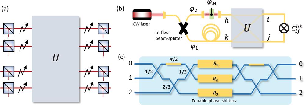
Optical losses deviate the interferometer operation from the unitarity. To take into account the losses, we consider biased insertion losses at the input and at collection stages and balanced internal losses, which are known to commute with the unitary matrix.40 This assumption is not the most general, since it considers the optical transformation U without any internal imbalances among the modes. Currently, most of the photonic circuits are designed in such a way that losses are practically unbiased along the evolution and can be factorized to one of the ends of the interferometer.25 Then our model of losses can find applications in many scenarios. We model losses as shown in Fig. 1(a) with a set of beam splitters placed on the input and output modes. We further consider the presence of unknown (and possibly unstable) phase terms on these modes. The device is thus described by a matrix T=D1UD2, where D1 and D2 are diagonal matrices that account for such losses and additional phases. The matrix elements of the unitary part are expressed as Uij=τijeiϕij, where τij and ϕij are the matrix moduli and phases, respectively. In what follows, we briefly analyze the two most general algorithms in the literature to reconstruct the matrix U. The first algorithm exploits quantum light,28 and the second one is based on coherent light measurements.30

If one employs measurements with Fock states at the input of the interferometer and photon-number-resolving detection at the output, the results will be insensitive to the (unstable) phase terms at the input and at the output. This means that the matrix U and all the matrices U′ in the form U′=F1UF2, where F1 and F2 are unitary diagonal matrices, and are equivalent. Another invariance property of these measurements carried out with Fock states is that the outcomes do not change with respect to the conjugate operation U′=U*. Given these equivalence relations, it is not necessary to reconstruct the actual unitary matrix implemented by the interferometer, but only a representative element of its class of equivalence. This is commonly defined by choosing a matrix with real-valued elements in the first row and first column (ϕ0i=0 and ϕi0=0) together with the condition that the element U11 has positive phase (ϕ11>0). Laing and O’Brien28 presented an algorithm to reconstruct the value of moduli and phases of the representative unitary matrix elements via single-photon intensity and two-photon measurements, the latter via the visibility V of HOM interference.37 Labeling the input modes of the two photons as h,k, and the output ones as i,j, the visibility is defined as Vijhk=1−(Pijhk)I(Pijhk)D=−2τjkτihτikτjhτjk2τih2+τik2τjh2cos(ϕjk+ϕih−ϕik−ϕjh),(2)where (Pijhk)I is the probability to find the two (indistinguishable) photons in output modes (i,j) when they are injected, respectively, in input modes (h,k), whereas (Pijhk)D correspond to the same quantity with distinguishable particles. Note that the visibility V does not change in the presence of mode-dependent losses in both preparation and measurement stages, and thus its estimation gives direct access to the matrix elements. By measuring these quantities, it is possible to define a system of equations and to retrieve an analytical solution to the problem, as shown in Refs. 28 and 29. One of the main constraints of such an approach is the requirement of measurement with quantum light. Recently, a further method that exploits quantum light probes, such as two-mode squeezed states, and single-photon counting combined with heterodyne measurements, provided further refinement for reconstructing the U matrix in the presence of internal unbalanced losses.41

The other method proposed in Ref. 30, based on classical intensity measurements, requires phase stability within the measurement time to estimate matrix phases, since these values are extracted from first-order correlation functions. This means that in such a measurement scheme, the equivalence between U and U′ does not hold. Additionally, the correct estimation of matrix element moduli, which in this approach is performed independently from the phase estimations, is spoiled by the presence of output mode-dependent losses.

In this section, we propose an alternative black-box methodology based on coherent light probes. This approach permits the estimation of matrix elements moduli and losses also in the presence of loss imbalance among the modes and retrieving quantities having the same properties of V without requiring phase stability at the inputs and outputs of the interferometer.

We start our investigation with the estimation of the matrix elements moduli τij. The τij2 coefficients represent the probability of finding a single photon in output mode j given an input mode i or, alternatively, the fraction of classical field intensity in the mode j. This observation allows one to define a probability matrix Pij=τij2. The main task is to estimate such a matrix when mode-dependent losses are present in the preparation and collection stages. Let us define M as the matrix obtained from single-mode intensity measurements, estimated experimentally via single-photon input states or by injecting laser light in a single mode. Following the model presented in Fig. 1(a), the actual measured matrix M can be expressed as M=D1PD2,(3)where D1 and D2 are the diagonal matrices that describe the unbalanced losses in input and output modes. The task then requires reconstructing the probability matrix P and the input and output losses matrices D1 and D2 starting from the measured matrix M. To this end, we now introduce below two approaches that can be used to estimate D1 and D2 up to a multiplicative factor and, consequently, matrix P under very few assumptions on the measured matrix M.

A first approach to reconstruct matrices P, D1, and D2 is obtained starting from the observation that the probability matrix P is a doubly stochastic matrix, i.e., the matrix has nonnegative entries and the sum of each row and each column is equal to 1. It is thus possible to apply Sinkhorn’s theorem and the matrix scaling algorithm on this system.42^,43 Indeed, a matrix with nonnegative elements such as M admits a Sinkhorn’s decomposition if it is diagonally equivalent to a doubly stochastic matrix, i.e., can be written in the form D1PD2, where D1 and D2 are the diagonal matrices and P is a doubly stochastic matrix. This decomposition exactly represents the solution to our problem [see Eq. (3)]. Sinkhorn’s theorem and subsequent extensions42 guarantee that this solution exists and it is unique. The theorem gives us also an important warning, since the algorithm is sensitive to the position of the zero elements of the measured matrix M. This means that an incorrect attribution of zero-valued elements in M, due to experimental errors or limited measurement sensitivity, could make the matrix impossible to decompose with Sinkhorn’s theorem.

Finding Sinkhorn’s decomposition for a nonnegative matrix M is a special case of the matrix scaling problem that has applications in a large variety of fields. In our case, defining X=D1−1 and Y=D2−1, we can write P=XMY and using the property that P has to be doubly stochastic, we obtain the following system of equations: {XMYe→=e→,YMTXe→=e→,(4)where e→ is the vector with all the components equal to 1.

In the literature, different algorithms have been proposed to solve Eq. (4). Here we present a specific choice among the possible algorithms (see Ref. 44 for a review of the possible approaches). The chosen algorithm allows the recovery of all three matrices in Eq. (3). The idea is to rearrange Eq. (4) in terms of vectors x→ and y→, which are the diagonal elements of X and Y. Formally, they can be expressed as x→=Xe→ and y→=Ye→. By defining the inversion of a vector as the inversion component-by-component, x→−1=(x1−1,x2−1,…,xN−1)T, we find that {x→=(My→)−1,y→=(MTx→)−1.(5)

At this point, we apply an iterative algorithm to solve the system of Eq. (5) and retrieve the two vectors x→ and y→ and, consequently, the two diagonal matrices X and Y. Then we can recover the probability matrix P=XMY and the two loss matrices as D1=X−1 and D2=Y−1.

In the derivation of the previous algorithm to solve Eq. (3), we have implicitly assumed to have measured the field intensity distribution for any combination of outputs j for any input i. In the following method, we define an alternative procedure that can be applied when only a subset of the inputs is available, while requiring the capability of reconfiguring the linear optical network.

Let us then consider an interferometer, in which it is possible to change the probability matrix P without affecting the input and output losses D2 and D1 and to measure all the output configurations only for a subset of input modes. We first consider the scenario, in which the light source, a single photon, or a laser beam, is injected only in mode i. In the absence of unbalanced losses, the outcome M→ of such intensity measurements is proportional to the vector P→, (the i’th column of the matrix P) and represents a discrete probability distribution that depends from a set of parameters θ→ describing the optical circuit settings. By taking into account the presence of unbalanced losses D→ (D1 in the general case), the components Mj of vector M→ are Mj(θ→)=IPj(θ→)Dj,(6)where I is the intensity attenuated by the input loss. Since we are injecting light in the same mode for all measurements, this factor can be included in D→.

The separation of the probability from the losses in Eq. (6) can be done starting from the following observation. Let us define the quantity S(α→,θ→) as the weighted sum of the components of M→, S(α→,θ→)=∑jαjMj(θ→).(7)

If the vector of the weights α→ is proportional to the element-wise inverse of the losses vector D→, the quantity S does not vary with the control parameter θ→. In fact, when α→=βD→−1, where β is a global factor, we have S(βD→−1,θ→)=β∑jDj−1Mj(θ→)=β∑jDj−1DjPj(θ→)=β.(8)

In general, S(α→,θ→) changes with the control parameters θ→. Then the idea is to find the weight vector α→ such that S(α→,θ→) is constant when the control parameters θ→ vary. This vector can be obtained by minimizing the variance of S(α→,θ→) with respect to α→. The variance ξ2(α→) can be estimated on a sufficiently large set of settings of the parameters {θ→i} as ξ2(α→)=∑i=0n−1S(α→,θ→i)2n−(∑i=0n−1S(α→,θ→i)n)2,(9)where n is the number of different settings {θ→i}, and consequently represent the size of the measurement outcome vector {M→(θ→i)}. This minimization is equivalent to a quadratic optimization problem. To solve such a task, let us call Mij=[M→(θ→i)]j the matrix in which each row contains the output intensities distribution for a particular configuration of the chip; then we define the following positive semidefinite matrix Q as Qhk=1n∑i=0n−1MihMik−1n2∑i=0n−1∑j=0n−1MihMjk.(10)

Then our problem can be rewritten, in terms of the matrix Q, as ξ2(α→)=∑i∑jQijαiαj.(11)

The minimization of Eq. (11) has as a trivial solution α→=0→ (the vector with all null components) and another one that is the eigenvector of Q corresponding to a null eigenvalue. The latter solution corresponds exactly to the element-wise inverse of the losses vector α→=D→−1. In the presence of noisy experimental data, the solution is the eigenvector of Q corresponding to the lowest eigenvalue. Alternatively, the nontrivial solution can be found by an ordinary numerical minimization approach of Eq. (11). This can be fulfilled by setting a normalization constraint N→·α→=1 for some normalization vector N→, since losses can be estimated with this procedure up to a multiplicative factor common to all the modes.

The method can be generalized to the scenario, in which one is interested in reconstructing a submatrix of P. Then it is possible to reconstruct even the relative losses between the different measured input modes. Here we suppose a set of output vectors {M→i}k for each input k∈K and compute the variance function ξk2(α→) and the associated matrix Q(k). At this point, we minimize the sum of all variances with the same constraints of the previous derivation, ∑k∈Kξk2(α→)=∑i∑j∑k∈KQij(k)αiαj.(12)

After the minimization, it is possible to recover the input losses from the value of the sum function associated with each input as follows: (D→2)k(D→2)k′=1n∑i=0n−1∑jαjMij(k)1m∑i=0m−1∑jαjMij(k′).(13)

Here we propose a procedure to estimate the complex phases of the matrix elements ϕij. The methods reported in Refs. 28 and 29 employ the visibility of the HOM effect described in Eq. (2) for this task, by sending a two-photon input state whose indistinguishability is tuned during the experiment. In this work, we propose an analogous quantity that can be measured by intensity cross-correlation at the output of the linear network with classical light. The measurement scheme is presented in Fig. 1(b). The laser source is split and sent into the network in modes (h,k). The additional phases φ1 and φ2 account for phase instabilities in the optical paths between the sources and the interferometer. We can define the cross-correlation σijhk between the output modes (i,j) when the two beams enter from modes (h,k) as σijhk=⟨(Ii−⟨Ii⟩)(Ij−⟨Ij⟩)⟩=⟨IiIj⟩−⟨Ii⟩⟨Ij⟩,(14)where Ii and Ij are the field intensities in the corresponding output modes, whereas ⟨·⟩ is the time average. We define also the self-correlation σiihk of the intensity fluctuation as σiihk=⟨(Ii−⟨Ii⟩)2⟩=⟨Ii2⟩−⟨Ii⟩2.(15)

We make the hypotheses that (i) the external phase fluctuations φ=φ1−φ2 have zero time average and (ii) the input laser intensity is constant. After some calculations, reported in Sec. II in the Supplementary Material, we can define the normalized cross-correlation Cijhk as Cijhk=σijhkσiihkσjjhk=cos(ϕih−ϕik−ϕjh+ϕjk).(16)

Note that this quantity only depends on the phase of the matrix elements. Similar to HOM visibility in two-photon experiments, the set {Cijhk} does not depend on the input and output losses. Additionally, and at variance with HOM visibility, {Cijhk} does not depend also on the moduli {τi,j} of the matrix elements, thus permitting an independent estimation of the phases. The derivation of Eq. (16) is performed under a specific assumption on the external optical phase fluctuations at the input. More specifically, we require that ⟨eιφ⟩=0⟨e2ιφ⟩=0.(17)

In general, mechanical and thermal phase fluctuations do not satisfy these conditions. These equations can be satisfied by adding a phase modulator in one of the two input paths. In this scenario, the external phase contribution can be expressed as φ=φM+φT, where φM is the modulated phase and φT is the one modified by thermal and mechanical noise. Since the two contributions are uncorrelated, we can write ⟨eιφ⟩=⟨eιφM⟩⟨eιφT⟩. Controlling the phase modulation such that ⟨eιφM⟩=0 and ⟨e2ιφM⟩=0, for example, by adding white noise with appropriate amplitude or by a discrete set of phases, the conditions of Eq. (17) can be satisfied.

Given the methods defined above, we can summarize the complete procedure to reconstruct the matrix U as follows:

Note that point 2 has some similarities to the procedure proposed in Refs. 28 and 29 with HOM visibilities. In particular, this approach could require a further minimization step on a larger set of {Cijhk} with respect to the minimum ensemble needed to solve the system. Nonetheless, it is worth noting that, in our case, we do not require (i) the use of indistinguishable single-photon states and (ii) the measurements of {Cijhk} give us directly the information about the phases without requiring the knowledge of the matrix moduli. In fact, in our algorithm, points 1 and 2 are independent, as for the previous methods with coherent probe light,30^,33 but have the additional features of permitting the estimation of losses. Furthermore, it can be applied in any scenario with phase instabilities.

We tested the complete algorithm described in the previous section in a three-mode reconfigurable optical circuit. The waveguides of the device were fabricated in a glass sample via the femtosecond laser-writing technique45 (see Sec. III in the Supplementary Material for more details). The structure is composed of a sequence of two tritters, a circuit that generalizes the beam splitter over three modes46^,47 [see also Fig. 1(c)]. Between the two tritters, the presence of three resistive heaters permits the change of the unitary transformation performed by the circuit via the thermo-optic effect. The measurements were performed with a continuous-wave (CW) laser at the wavelength of λ=785nm. The laser is routed in different input modes via a fiber switch connected to a fiber array that injects light into the input port of the interferometer. The field intensity distribution in the three output ports was recorded via a CCD camera.

Our first experimental test regards the two algorithms described above, to retrieve the losses vectors and moduli of the matrix elements. In Figs. 2(a) and 2(b), we report the results for the application of Sinkhorn’s decomposition method. In particular, in (a), we report the measured field intensity M for a particular configuration of the chip, normalized to the column total intensity. Here we inserted on-purpose additional losses by placing an attenuation filter on the output mode 0, to test the performances of the approach. In Fig. 2(b), we report the probability matrix P after the applications of the Sinkhorn algorithm. We measured the moduli of a set of N different transformations U, each of them in two loss conditions, namely, by inserting and removing the attenuation filter in mode 0. Defining the fidelity as F=(1/3∑i,j=02PijPij′)2, the average classical similarity between the two reconstructed distributions in the two losses configurations for a given U via the Sinkhorn method is F‾=0.9999±0.0001 (Fmin=0.9997). The average was estimated on the set of the N pairs of matrices. This confirms that the method works properly in different mode-dependent loss configurations and retrieves, as expected, always the same moduli |τi,j|2 associated with the transformation U.

We then move to test the second algorithm based on variance minimization. In Fig. 2(c), we report the measured field intensity in the three outputs of the interferometer for different dissipated powers in one heater, thus corresponding to different evolutions of U, when the signal is injected in input 0. We also report the sum (red curve) of the three intensities for each tested configuration for U. We observe that such a sum is not constant, as one would expect if the output losses were balanced. In Fig. 2(d), we report the same curves after applying the variance minimization algorithm, showing that the application of the algorithm makes the sum constant with respect to changes in the internal transformation. We repeat the same procedure of the previous paragraph by tuning the output mode-dependent losses, showing the capability of retrieving the correct moduli values. The average fidelity, among the same set of N internal operations, between the reconstructed distributions in the two different conditions of losses after the application of the algorithm is F¯=0.9996±0.0002 (Fmin=0.9990). As a further confirmation, we compared the distributions, corresponding to the same optical circuit settings, retrieved by the application of the two algorithms. The mean fidelity between the reconstructed matrix with the two methods is F¯=0.999±0.001 (Fmin=0.992), thus confirming the effectiveness of both algorithms.

Finally, we tested the measurement of the cross-correlations defined in Eq. (16) for the phase reconstruction. Since the phase fluctuations of the fibers do not fulfill the conditions of Eq. (17), we placed a liquid crystal in one arm before the first input of the photonic chip. For the phase modulation, we used a discrete set of phases instead of a continuous one. In particular, we employed the set {0,2π/3,4π/3}. After recording the temporal fluctuations of the output field intensities, we calculated the normalized cross-correlations for various configurations of the interferometer (red dot in Fig. 3). These measurements are compared with the predictions made by an independent characterization of the device via a white-box algorithm, used as a reference to test our approach. By this alternative method, which exploits the structure of the two tritters, the moduli and the phases of the matrix are retrieved directly from the field intensity distributions of the previous paragraph. It follows that, in this white-box approach used as a reference, the cosines of the internal phases are the result of a numerical optimization between the parameters of the optical circuit, which is designed according to the structure in Fig. 1(c) and the measurements of the P→ distributions. The blue curve in Fig. 3 represents the prediction of such an optimization. We observe that the direct measurement of cross-correlation via the proposed approach with classical light and the same quantities retrieved via the white-box method are compatible with the experimental error, with a normalized χ2=1.09. As a final comparison, we compute the fidelity between the second column of the matrix retrieved via our black-box algorithm (bb) Ui1bb and the column of the white-box approach (wb) Ui1wb. We choose the second column of the matrix, since it presents nontrivial phases, namely, ϕi1≠0 for i>0. Indeed, the first row and column are imposed to be real vectors because of the equivalence between U and U′=F1UF2 with F1 and F2 unitary diagonal matrices. The fidelity defined here as F=|∑i=02Ui1bb(Ui1wb)*|2, i.e., the overlap between pure single-photon states described by the second column of U, has been estimated for each configuration of the dissipated power in R1 reported in Fig. 3. The average fidelity is F¯=0.999±0.001 (Fmin=0.994).

In this work, we presented algorithms to characterize the operation of multimode linear optical circuits. In particular, we have shown the possibility of reconstructing the moduli of the unitary matrix element by field intensity measurements, in the presence of unbalanced losses at the input and output ports. This is in contrast to the previous black-box algorithms28^,29 that can reconstruct the moduli of the matrix only after phases measurements via HOM visibility and by imposing the constraint to have a unitary matrix. In addition, our procedure can provide directly the differential losses among the waveguides at the input and output. We also proposed a method to characterize the internal matrix phases based on intensity correlations of coherent light beams at the outputs of the linear network. These measurement methods do not require knowledge of the matrix moduli and of input/output losses. These approaches enable the possibility of characterizing separately the moduli and the phases of the unitary matrix implemented by the optical network with a reliable and independent approach. Furthermore, all presented algorithms are polynomial in the number of modes of the interferometer, both for the execution time and for the number of measurements required, sharing the same scaling of previous state-of-the-art algorithms. This property makes our algorithms suitable for adaption to large-scale interferometers. An open issue regards the inclusion of unbalanced internal losses in the model. Some recent works have proposed some solutions for taking into account such sources of noise in the U reconstruction.41 We foresee as a future purpose of our work to adopt the same strategy of independent estimations of moduli and phases to detect the effects of such imperfections. We provided experimental proof of the effectiveness of the algorithm by verifying its performance on a three-mode reconfigurable integrated optical circuit. In this analysis, we compared the results with the predictions of an independent reconstruction that exploits the knowledge of the internal structure of the circuit, which may be in general unknown or too complex to model when taking into account noise processes.

Our findings pave the way for the successful adoption of such an effective black-box methodology to large-scale optical networks, which nowadays are approaching a high number of optical modes and components,19^,22^,23 with applications ranging from quantum communication and sensing to quantum computation and simulation via photonic systems.

Francesco Hoch received his master’s degree in 2019. He is currently a PhD student in the Physics Department of Sapienza University. His research interest focuses on reconfigurable integrated optics and their application for quantum information and quantum computation. In particular, he worked on the development of new reconfigurable devices for the boson sampling experiment and the study of the optical implementation of recently proposed quantum protocols.

Taira Giordani received her PhD in physics in 2020. She is currently a postdoc in the Physics Department of Sapienza University. Her research focuses on the experimental implementation of quantum walks in integrated photonic devices and the angular momentum of light. In this context, her efforts aim to develop machine learning and optimization methods for the certification and engineering of photonic quantum walk platforms.

Nicolò Spagnolo received his PhD in 2012 in physical sciences of matter with a thesis on experimental multiphoton quantum optical states. He is currently tenure-track assistant professor in the Physics Department of Sapienza Università di Roma. His research interests are focused on quantum information protocols employing different photonic platforms. These research activities include the implementation of boson sampling instances and of validation protocols with integrated photonics, quantum phase estimation experiments, and optical quantum communications.

Andrea Crespi received his PhD in physics from the Politecnico di Milano, Italy, in 2012. From 2012 to 2016, he worked as a research fellow at the Institute for Photonics and Nanotechnologies of the National Research Council. Since 2016, he has been in the Physics Department of Politecnico di Milano, where he is now an associate professor. His research interests include femtosecond laser micromachining of glass and the development of integrated photonics circuits for quantum photonics applications.

Roberto Osellame received his PhD in physics from the Politecnico di Torino in 2000. He is a research director at the Institute for Photonics and Nanotechnologies of the National Research Council, Milan, Italy. His research interests focus on microfabrication of integrated photonic devices for quantum technologies, lab-on-a-chip, and optical communications. He is a co-author of more than 300 publications and holds 15 patents. He is a fellow of Optica and an ERC awardee.

Fabio Sciarrino received his PhD in 2004 with a thesis in experimental quantum optics. He is a full professor and a head of the Quantum Lab in the Department of Physics of Sapienza Università di Roma. Since 2013, he has been a fellow of the Sapienza School for Advanced Studies. His main field of research is quantum information and quantum optics, with works on quantum teleportation, optimal quantum machines, fundamental tests, quantum communication, and orbital angular momentum.