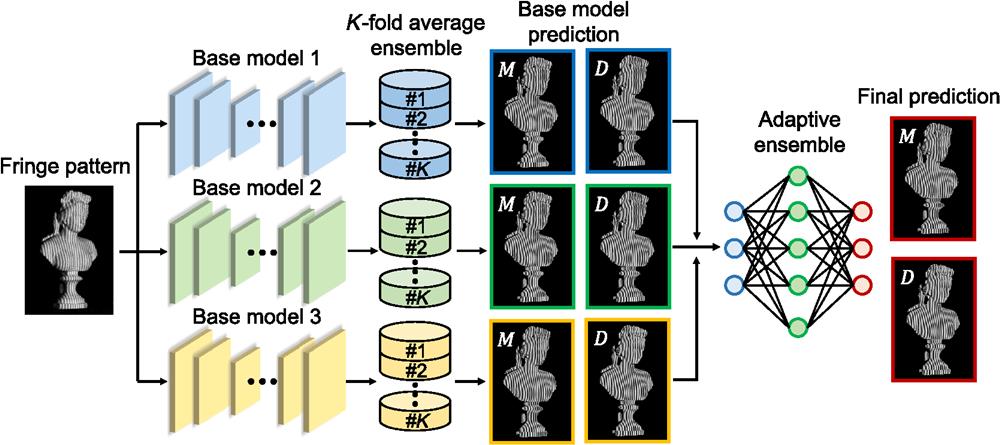
Fig. 1. Diagram of the fringe-pattern analysis using ensemble deep learning. The input fringe image is processed by three base models. In each base model, a K-fold average ensemble is proposed to generate K sets of data to train K homogeneous models. Each homogeneous model outputs a pair of numerator M and denominator D. The mean is computed over K homogeneous models and is treated as the output of the base model. To further combine the predictions of the base models, an adaptive ensemble is developed that trains a DNN to fuse their predictions adaptively and gives the final prediction.

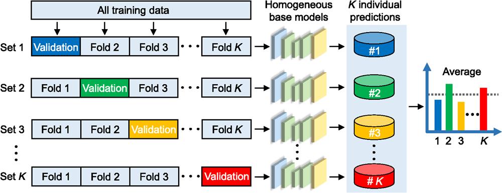
Fig. 2. Diagram of the K-fold average ensemble approach. The whole data set is equally separated into K parts. We combine any K−1 parts of the data for training and leave the remaining part for validation. Then, K sets of data can be generated to train a base model, which yields K homogeneous models. Each one gives a prediction independently, and their average is calculated as the output of the K-fold average ensemble.

Fig. 3. Diagram of the proposed adaptive ensemble. (a) It trains a MultiResUNet to combine the predictions of base models. (b) Structure of the MultiRes block, where a series of 3×3 convolutions is used to approximate the behaviors of 5×5 convolution and 7×7 convolution. (c) Structure of the residual path, where features of the encoder pass through a few convolutional layers before being fed into the decoder.

Fig. 4. Experimental results of several unseen scenarios that include a set of statues, an industrial part, and a desk fan. The input is a fringe pattern. It is then fed into the U-Net, MP DNN, and Swin-Unet, which are trained by the sevenfold average ensemble, respectively. By calculating the average, each base model outputs a pair of numerators and denominators. Then, the outputs of base models are processed by the adaptive ensemble, which combines the contribution of each base model and calculates the wrapped phase.

Fig. 5. Comparison of the proposed method with the U-Net. (a) and (b) The absolute phase error maps of the U-Net and our method, respectively. (c) Selected ROIs of the phase error for the two methods. (d) The performance of different K-fold average ensembles.

Table 1. Quantitative validation of the proposed approach.