Fringe-pattern analysis with ensemble deep learning

Shijie Feng; Yile Xiao; Wei Yin; Yan Hu; Yixuan Li; Chao Zuo; Qian Chen

doi:10.1117/1.APN.2.3.036010

Abstract

In recent years, there has been tremendous progress in the development of deep-learning-based approaches for optical metrology, which introduce various deep neural networks (DNNs) for many optical metrology tasks, such as fringe analysis, phase unwrapping, and digital image correlation. However, since different DNN models have their own strengths and limitations, it is difficult for a single DNN to make reliable predictions under all possible scenarios. In this work, we introduce ensemble learning into optical metrology, which combines the predictions of multiple DNNs to significantly enhance the accuracy and reduce the generalization error for the task of fringe-pattern analysis. First, several state-of-the-art base models of different architectures are selected. A K-fold average ensemble strategy is developed to train each base model multiple times with different data and calculate the mean prediction within each base model. Next, an adaptive ensemble strategy is presented to further combine the base models by building an extra DNN to fuse the features extracted from these mean predictions in an adaptive and fully automatic way. Experimental results demonstrate that ensemble learning could attain superior performance over state-of-the-art solutions, including both classic and conventional single-DNN-based methods. Our work suggests that by resorting to collective wisdom, ensemble learning offers a simple and effective solution for overcoming generalization challenges and boosts the performance of data-driven optical metrology methods.

Keywords

deep learning ensemble learning fringe-pattern analysis optical metrology phase retrieval three-dimensional measurement

Video Introduction to the Article

1 Introduction

Optical metrology plays a significant role in many fields because of its merits of noninvasiveness, flexibility, and high accuracy. In optical metrology, fringe-pattern analysis is indispensable to many tasks, e.g., interferometry, fringe projection profilometry, and digital holography. According to the number of patterns used, fringe-pattern analysis can be generally classified into two categories: single-frame and multiframe methods. The Fourier-transform fringe-pattern analysis is a representative single-frame approach1 that converts a fringe pattern into the frequency domain and extracts the phase information by filtering the first order of the spectrum. This method is suitable for measuring dynamic scenes because it only needs a single fringe image. However, it tends to compromise on handling complex surfaces, owing to the spectrum aliasing issue. In contrast, the multiframe approaches, e.g., the $N$ -step phase-shifting (PS) algorithm,2 can achieve higher accuracy, since the phase demodulation can be carried out pixel by pixel along the temporal axis. Nevertheless, multiframe approaches usually suffer when facing fast-moving objects because of the need to capture multiple images. Hence, there is a contradiction between the efficiency and the accuracy of the fringe-pattern analysis.

Recently, many advances have emerged in the field of optical metrology that benefit from harnessing the power of deep learning.3^,4 Fringe-pattern analysis using deep learning has shown promising performance in measuring complex contours using a single fringe image.5 As a data-driven approach, it can exploit useful hidden clues that may be overlooked by traditional physical models, thus showing potential for resolving the contradiction between efficiency and accuracy in the phase demodulation. However, it is not trouble-free for this kind of approach. Usually, people adopt a single deep neural network (DNN) and depend on it completely to handle all possible measurements once it is trained. Actually, this is risky, as the DNN may only learn limited attributes of input data because of its fixed structure. Consequently, it tends to demonstrate high variance for unseen scenarios. Further, the DNN may converge to a local loss minimum during training, which further increases the risk of making unreliable predictions.

To handle these issues, ensemble deep learning has been developed,6^,7 which refers to a set of strategies where, rather than relying on a single model, several base models are combined to perform tasks. As different architectures can capture distinct information, better decisions can be made by combining different networks. Inspired by recent successful applications of ensemble deep learning, we demonstrate for the first time, to the best of our knowledge, that an ensemble of multiple deep-learning models can improve the accuracy and the stability of fringe-pattern analysis substantially. First, multiple state-of-the-art DNNs for fringe-pattern analysis are employed as base models. To train the base models, we propose a $K$ -fold average ensemble method to divide training data into several groups so that each one can be trained multiple times by using different data. Then, the average of the predictions is calculated as the output of each base model. To further fuse the outputs of the base models, we develop an adaptive ensemble that trains an extra DNN to extract and combine useful features from these outputs adaptively and automatically during training. Experimental results show that the proposed approach can improve the phase accuracy and the generalization capability for unseen scenarios greatly compared with the traditional method using a single model.

Sign up for Advanced Photonics Nexus TOC. Get the latest issue of Advanced Photonics Nexus delivered right to you！Sign up now

2 Methods

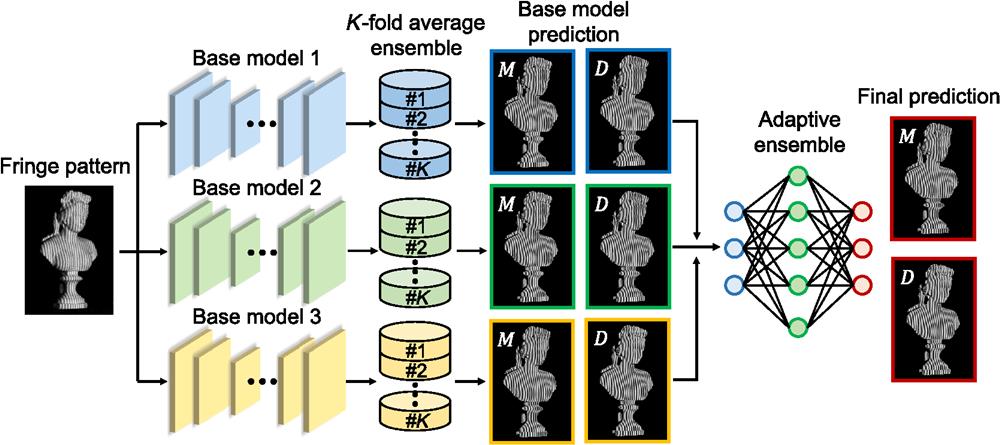
In fringe-pattern analysis, a fringe image is often written as $I (x, y) = A (x, y) + B (x, y) \cos φ (x, y),$ (1)where $(x, y)$ is the pixel coordinate, $A$ is the background signal, $B$ is the amplitude, and $φ$ is the phase to be measured. Conventionally, the phase is demodulated through an arctangent function, $φ (x, y) = \arctan \frac{c B (x, y) \sin φ (x, y)}{c B (x, y) \cos φ (x, y)} = \arctan \frac{M (x, y)}{D (x, y)},$ (2)where the numerator $M$ represents the phase sine $[\sin φ (x, y)]$ and the denominator $D$ represents the phase cosine $[\cos φ (x, y)]$ . $c$ is a constant that is determined according to the phase demodulation approach. According to Eq. (2), a DNN can be constructed to learn to predict $M$ and $D$ . Then, the phase $φ$ can be computed through the arctangent function.5

Instead of relying on a single model, we train several base models to analyze the same input fringe image and combine their outputs as the final prediction. Figure 1 demonstrates the diagram of the proposed framework. First, three state-of-the-art models for fringe-pattern analysis are selected as base models. The first two models are the U-Net8 and the multipath DNN (MP DNN),5 which are convolutional neural networks that are good at extracting local features. The third model is the Swin–Unet,9 which is a vision transformer that shows the advantage of capturing global information. The structures of base models are detailed in the Supplementary Material. As these models have different architectures, diverse attributes of the input data can be learned. To train the base models, we develop a $K$ -fold average ensemble, whose schematic is shown in Fig. 2. The whole training data set is divided into $K$ parts equally (i.e., from fold 1 to fold $K$ ). Any $K - 1$ parts of the data can be merged and then used for training; the remaining one is used for validation. In this way, we can generate $K$ sets of training data. As each of them is different, additional information can be provided. To train these base models, we use the following mean squared error loss function: $Loss (θ^{i}) = \frac{1}{H \times W} \sum_{h = 1}^{H} \sum_{w = 1}^{W} {(y_{h, w}^{i} - {\hat{y}}_{h, w}^{i})}^{2},$ (3)where $θ^{i}$ represents the parameters of the $i$ th base model; these are learned during the training process. $H$ and $W$ represent the height and width of the image in pixels, respectively. Omitting the pixel index, $y^{i}$ is the output of the base model that consists of a pair of estimated numerator and denominator. ${\hat{y}}^{i}$ is the ground-truth label that can be obtained by the PS algorithm. With the $K$ -fold average ensemble, $K$ homogeneous models can be trained for each base model. As each homogeneous model can give a prediction, $K$ pairs of predictions can be obtained. In this work, the structures of these homogeneous models are the same. We use the He normal initialization to initialize the parameters of these networks.10 As both the training data and the initial values of the parameters are different, the performance of each network will be different, which enhances the diversity in model prediction. To combine these predictions, their average is computed as ${\bar{y}}^{i} = \frac{1}{K} \sum_{k = 1}^{K} y_{k}^{i},$ (4)where $y_{k}^{i}$ is the prediction of the $k$ th homogeneous model regarding to the $i$ th base model and ${\bar{y}}^{i}$ is the output of the $i$ th base model using the $K$ -fold average ensemble.

Figure 1.Diagram of the fringe-pattern analysis using ensemble deep learning. The input fringe image is processed by three base models. In each base model, a $K$ -fold average ensemble is proposed to generate $K$ sets of data to train $K$ homogeneous models. Each homogeneous model outputs a pair of numerator $M$ and denominator $D$ . The mean is computed over $K$ homogeneous models and is treated as the output of the base model. To further combine the predictions of the base models, an adaptive ensemble is developed that trains a DNN to fuse their predictions adaptively and gives the final prediction.

Figure 2.Diagram of the $K$ -fold average ensemble approach. The whole data set is equally separated into $K$ parts. We combine any $K - 1$ parts of the data for training and leave the remaining part for validation. Then, $K$ sets of data can be generated to train a base model, which yields $K$ homogeneous models. Each one gives a prediction independently, and their average is calculated as the output of the $K$ -fold average ensemble.

To further combine the predictions of the base models, we develop an adaptive ensemble that adopts a MultiResUNet to fuse the features of different models adaptively.11 The diagram of the adaptive ensemble is shown in Fig. 3. The feature extraction is enhanced by MultiRes blocks that use a series of $3 \times 3$ convolutions, as shown in Fig. 3(b). This structure is equivalent to the $5 \times 5$ and $7 \times 7$ convolutions and has the advantage that it can not only learn features of various base predictions at different image scales but also saves memory and speeds up network training. In addition, instead of combining the features of encoders and decoders immediately, residual paths are constructed, where features of the encoder are processed by several convolutional layers, which can reduce the content gap between encoder and decoder features. To train the MultiResUNet, we also use the loss function shown in Eq. (3). During training, the MultiResUNet can learn proper weights for features extracted from each base prediction without manual intervention, thus making the fusion in an adaptive and automatic way.

Figure 3.Diagram of the proposed adaptive ensemble. (a) It trains a MultiResUNet to combine the predictions of base models. (b) Structure of the MultiRes block, where a series of $3 \times 3$ convolutions is used to approximate the behaviors of $5 \times 5$ convolution and $7 \times 7$ convolution. (c) Structure of the residual path, where features of the encoder pass through a few convolutional layers before being fed into the decoder.

3 Results

We validated the presented method under the scenario of fringe projection profilometry. The system consists of a camera (V611, Vision Research Phantom) and a projector (DLP 4100, Texas Instruments). The measured scene was illuminated by the projector with a sinusoidal fringe pattern, and the fringe image was captured by the camera from a different viewing point. To collect the training data, many fringe images of various objects were captured. To generate the ground-truth labels, the 12-step PS algorithm was applied. The captured fringe patterns are 8-bit gray-scale images. In the data preprocessing stage, the input fringe pattern was divided by 255 for normalization before being fed into the DNNs. Further details about the optical setup and the calculation of the ground-truth data are provided in the Supplementary Material. For the adaptive ensemble, the training data were generated using the trained base models. All base models and the MultiResUNet were implemented by the Keras and computed on a graphic card (GTX Titan, NVIDIA).

To test the performance of our approach, we measured three different scenarios that were not seen by these networks during training. They are a set of statues, an industrial part made of aluminium alloy, and a desk fan made of plastic. The experimental results regarding each stage of our approach are shown in Fig. 4. Here, for better performance, a seven-fold average ensemble was used to train each base model. So, we divided the training data into seven parts and trained seven homogeneous models for each base model. Given an input fringe pattern, the homogeneous models gave predictions independently, and Eq. (4) was used to compute the average. As there were three base models, three pairs of numerators and denominators were obtained for each input image. These predictions were further combined by being fed into the adaptive ensemble that output the final prediction and calculated the wrapped phase.

Figure 4.Experimental results of several unseen scenarios that include a set of statues, an industrial part, and a desk fan. The input is a fringe pattern. It is then fed into the U-Net, MP DNN, and Swin-Unet, which are trained by the sevenfold average ensemble, respectively. By calculating the average, each base model outputs a pair of numerators and denominators. Then, the outputs of base models are processed by the adaptive ensemble, which combines the contribution of each base model and calculates the wrapped phase.

For quantitative analysis, the ground-truth phase was obtained by the 12-step PS method. For comparison, the fringe image was also analyzed by a single U-Net; its absolute phase error is shown in Fig. 5(a). For the first scenario, we can see that the phase of smooth areas is retrieved accurately, while that of complex regions is measured with large errors. The mean absolute error (MAE) of the whole scene is 0.085 rad. The phase error of our approach is shown in Fig. 5(b). As can be seen, the phase error of the first scene has been reduced effectively. For detailed investigation, two regions of interest (ROIs), i.e., two complex regions around hairs, were selected. We can see that our method performs much better than the U-Net for handling the complex areas of depth variations and edges. Quantitatively, the MAE was greatly reduced to 0.061 rad when our method was used. For the second scenario, the MAE of the U-Net is 0.076 rad, and obvious errors can be observed around the edges and the small raised letters on the surface of the object, as can be seen in Figs. 5(b) and 5(c). When our approach was applied, these phase errors were apparently reduced, and the MAE of the scene has been reduced to 0.054 rad. Last, for the third scenario, our method also outperformed the U-Net, as the MAE decreased significantly from 0.080 to 0.059 rad, demonstrating the accuracy improvement by 26%.

Figure 5.Comparison of the proposed method with the U-Net. (a) and (b) The absolute phase error maps of the U-Net and our method, respectively. (c) Selected ROIs of the phase error for the two methods. (d) The performance of different $K$ -fold average ensembles.

To further validate the proposed method, we investigated the effect of the ensemble size of the $K$ -fold average ensemble. Different $K$ were tested for these base models; the results are shown in Fig. 5(d). We find that a similar trend can be observed for these base models. The MAE decreases with the increase of $K$ , and it tends to be stable when $K$ is larger than seven. Therefore, the sevenfold average ensemble was used in our work. Moreover, we also compared the accuracy of each base model under the cases of the single model and the seven-fold average ensemble. Table 1 shows their MAEs for the tested scenarios. From the performance of a single DNN, we find different models demonstrate different performances. For example, the U-Net shows the smallest MAE for the third scenario, while the MAE for the second scenario is the largest among the three models. When the seven-fold average ensemble was utilized, the ensembles outperformed the single model as the MAEs were reduced. After further combining the outputs of the base models by the adaptive ensemble, we obtained the smallest MAE of 0.061, 0.054, and 0.059 rad for these scenes, respectively. From this experiment, we can see that different DNNs have different advantages, and it is hard for a single DNN to demonstrate excellent performance for all scenarios. It is worth noting that the model accuracy and generalization capability can be improved significantly by the proposed approach, which combines the strengths of diverse models. More experimental results are provided in the Supplementary Material.


Method	MAE of #1 (rad)	MAE of #2 (rad)	MAE of #3 (rad)
U-Net (single)	0.085	0.076	0.080
MP DNN (single)	0.089	0.074	0.085
Swin-Unet (single)	0.081	0.075	0.081
U-Net (seven-fold)	0.072	0.065	0.067
MP DNN (seven-fold)	0.074	0.062	0.072
Swin-Unet (seven-fold)	0.069	0.063	0.067
Adaptive ensemble	0.061	0.054	0.059

Table 1. Quantitative validation of the proposed approach.

View all Tables

4 Conclusions

In this work, we have proposed a novel fringe-pattern analysis method using ensemble deep learning, which can exploit the contributions of multiple state-of-the-art DNNs. The $K$ -fold average ensemble approach is developed to manipulate the training data set into different groups. Each base model is trained several times with different groups of data. Within each base model, the output is computed by taking the average over the predictions of all homogeneous models. To further fuse the predictions of the base models, we have proposed an adaptive ensemble that can train a DNN to combine these predictions adaptively and automatically. Experimental results have shown that our work can leverage the strength of multiple base models to boost performance, which is superior to the method that only uses a single DNN. Furthermore, deepp-learning techniques have been widely applied in various optical metrology applications, such as phase unwrapping, 3D reconstruction, and image denoising. However, a single model with a fixed architecture may only extract limited information from input data. We believe that the idea of utilizing the collective wisdom demonstrated here can also be extended to these applications because more DNNs of different structures can extract diverse information from input data, which is advantageous for making reliable predictions. We believe this work has great potential in inspiring powerful and practical optical metrology techniques in the future.

Shijie Feng received his PhD in optical engineering at Nanjing University of Science and Technology. He is working as an associate professor at Nanjing University of Science and Technology. His research interests include phase measurement, high-speed 3D imaging, fringe projection, machine learning, and computer vision.

Yile Xiao is pursuing his MS degree at Nanjing University of Science and Technology. His research interests include phase measurement, high-speed 3D imaging, fringe projection, and deep learning.

Wei Yin received his PhD from Nanjing University of Science and Technology. His research interests include deep learning, high-speed 3D imaging, fringe projection, and computational imaging.

Yan Hu received his PhD from Nanjing University of Science and Technology. His research interests include high-speed microscopic imaging, 3D imaging, and system calibration.

Yixuan Li is a PhD student at Nanjing University of Science and Technology. Her research interests include phase measurement, high-speed 3D imaging, fringe projection, and deep learning.

Chao Zuo received his BE and PhD degrees from Nanjing University of Science and Technology (NJUST) in 2009 and 2014, respectively. He was working as a research assistant at the Centre for Optics and Lasers Engineering, Nanyang Technological University, from 2012 to 2013. Currently, he is working as a professor in the Department of Electronic and Optical Engineering and principal investigator of the Smart Computational Imaging Laboratory, NJUST. His research interests include computational imaging and high-speed 3D sensing and has authored over 160 peer-reviewed journal publications. He has been selected for the Natural Science Foundation of China for Excellent Young Scholars and the Outstanding Youth Foundation of Jiangsu Province, China. He is the fellow of SPIE and Optica.

Qian Chen received his BS, MS, and PhD degrees from Nanjing University of Science and Technology. Currently, he is working as a professor and vice-principal at Nanjing University of Science and Technology. He has been selected as Changjiang Scholar Distinguished Professor. With broad research interests in photoelectric imaging and information processing, he has authored more than 200 journal papers. His research team develops novel technologies and systems for non-interferometric quantitative phase imaging and high-speed 3D sensing and imaging with particular applications in national defense, industry, and bio-medicine.

References

[1] M. Takeda, K. Mutoh. Fourier transform profilometry for the automatic measurement of 3-D object shapes. Appl. Opt., 22, 3977-3982(1983).

[2] C. Zuo et al. Phase shifting algorithms for fringe projection profilometry: a review. Opt. Lasers Eng., 109, 23-59(2018).

[3] G. Barbastathis, A. Ozcan, G. Situ. On the use of deep learning for computational imaging. Optica, 6, 921-943(2019).

[4] C. Zuo et al. Deep learning in optical metrology: a review. Light: Sci. Appl., 11, 39(2022).

[5] S. Feng et al. Fringe pattern analysis using deep learning. Adv. Photonics, 1, 025001(2019).

[6] M. A. Ganaie et al. Ensemble deep learning: a review. CoRR(2021).

[7] M. S. S. Rahman et al. Ensemble learning of diffractive optical networks. Light: Sci. Appl., 10, 14(2021).

[8] O. Ronneberger, P. Fischer, T. Brox. U-net: convolutional networks for biomedical image segmentation. Lect. Notes Comput. Sci., 9351, 234-241(2015).

[9] H. Cao et al. Swin-unet: Unet-like pure transformer for medical image segmentation(2021).

[10] K. He et al. Delving deep into rectifiers: surpassing human-level performance on imagenet classification, 1026-1034(2015).

[11] N. Ibtehaz, M. S. Rahman. MultiResUNet: rethinking the U-Net architecture for multimodal biomedical image segmentation. Neural Networks, 121, 74-87(2020).