Deep learning reconstruction enables full-Stokes single compression in polarized hyperspectral imaging

Axin Fan; Tingfa Xu; Geer Teng; Xi Wang; Chang Xu; Yuhan Zhang; Xin Xu; Jianan Li

doi:10.3788/COL202321.051101

Abstract

Polarized hyperspectral imaging, which has been widely studied worldwide, can obtain four-dimensional data including polarization, spectral, and spatial domains. To simplify data acquisition, compressive sensing theory is utilized in each domain. The polarization information represented by the four Stokes parameters currently requires at least two compressions. This work achieves full-Stokes single compression by introducing deep learning reconstruction. The four Stokes parameters are modulated by a quarter-wave plate (QWP) and a liquid crystal tunable filter (LCTF) and then compressed into a single light intensity detected by a complementary metal oxide semiconductor (CMOS). Data processing involves model training and polarization reconstruction. The reconstruction model is trained by feeding the known Stokes parameters and their single compressions into a deep learning framework. Unknown Stokes parameters can be reconstructed from a single compression using the trained model. Benefiting from the acquisition simplicity and reconstruction efficiency, this work well facilitates the development and application of polarized hyperspectral imaging.

Keywords

deep learning reconstruction full-Stokes single compression polarized hyperspectral imaging

1. Introduction

Due to the rich information reflected, polarized hyperspectral imaging has been widely applied in environmental monitoring^[1], biological diagnosis^[2], food safety^[3], and other fields. In terms of technological development, polarized imaging is mainly based on Fourier transform^[4], pixelated polarizers^[5], and compressive sensing (CS)^[6]. Currently, all the above three methods can achieve full-Stokes polarized imaging.

Typically, Fourier transform imaging spectropolarimetry based on polarization modulation array (PMAFTISP)^[7] requires only one acquisition to obtain full-Stokes images. The PMAFTISP includes three polarization modulation arrays and three independent optical elements. System complexity and channel crosstalk may affect imaging quality. In addition, pixelated full-Stokes polarimeters require rotating polarizers^[8] or designing metasurfaces^[9,10]. Moreover, the fabrication of precision pixelated devices is costly and time-consuming.

Recently, compressive full-Stokes polarimeters are constructed with only two commercial components, providing an easy-to-operate and time-saving system. Full-Stokes images can be reconstructed from two measurements compressed by a quarter-wave plate (QWP) and a liquid crystal tunable filter (LCTF)^[11–13]. Furthermore, benefiting from a retarder followed by a Wollaston prism with a splitting effect, full-Stokes images can be reconstructed from one measurement^[14]. Nevertheless, the above compressive polarimeters all rely on traditional reconstruction methods, such as the two-step iterative shrinkage/threshold (TwIST) algorithm^[15], which require careful selection of polarization parameters and sparse basis.

Sign up for Chinese Optics Letters TOC. Get the latest issue of Chinese Optics Letters delivered right to you！Sign up now

This work develops full-Stokes single compression in polarized hyperspectral imaging by introducing deep learning reconstruction (DL-FSCPHI). Full-Stokes images are compressed by a QWP and an LCTF into only one measurement. In addition, the deep learning method can efficiently reconstruct full-Stokes images in one step, avoiding sparse basis selection.

2. DL-FSCPHI Method Overview

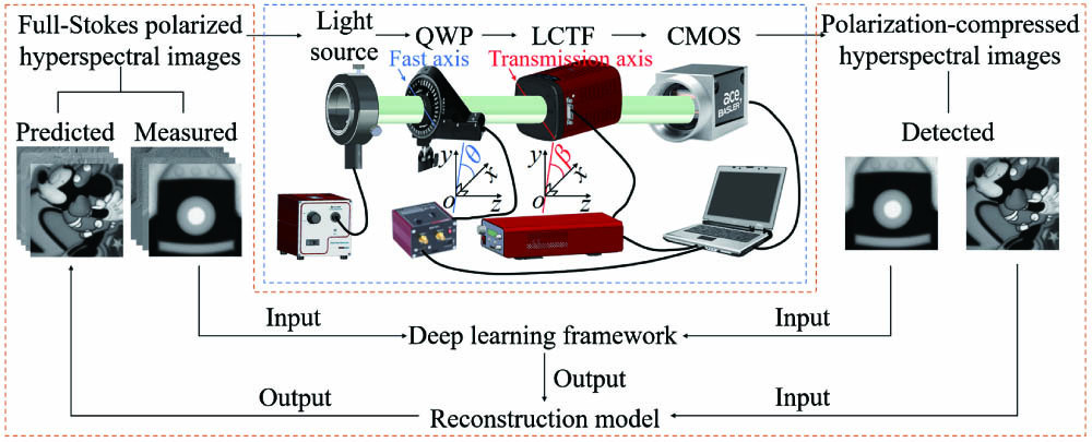
Figure 1 illustrates the overall schematic diagram of the DL-FSCPHI method comprising imaging system and polarization reconstruction. The imaging system mainly consists of a light source (Thorlabs, OSL2), a QWP (Thorlabs, SAQWP05M-700), an LCTF (Thorlabs, KURIOS-VB1/M), and a complementary metal oxide semiconductor (CMOS) detector (Basler, acA2040-180km). The polarization state of light can be expressed by four Stokes parameters. The polarization characteristics of an optical device can be described by a Mueller matrix with 16 elements in four rows and four columns. The interaction between light and optical devices is then reflected in the fact that optical devices can adjust the polarization state of light. Mathematically, the Mueller matrix of an optical device is multiplied by the four Stokes parameters of the input light to obtain the four Stokes parameters of the output light.

Figure 1.Overall schematic diagram of DL-FSCPHI method.

The Mueller matrices of the QWP and the LCTF are respectively expressed as $M_{Q} = [\begin{matrix} 1 & 0 & 0 & 0 \\ 0 & \cos^{2} (2 θ) & \cos (2 θ) \sin (2 θ) & - \sin (2 θ) \\ 0 & \cos (2 θ) \sin (2 θ) & \sin^{2} (2 θ) & \cos (2 θ) \\ 0 & \sin (2 θ) & - \cos (2 θ) & 0 \end{matrix}],$ (1) $M_{LC} = \frac{1}{2} [\begin{matrix} 1 & \cos (2 β) & \sin (2 β) & 0 \\ - \cos (2 β) & - \cos^{2} (2 β) & - \cos (2 β) \sin (2 β) & 0 \\ - \sin (2 β) & - \cos (2 β) \sin (2 β) & - \sin^{2} (2 β) & 0 \\ 0 & 0 & 0 & 0 \end{matrix}],$ (2)where $θ (0^{°} \leq θ \leq 180^{°})$ represents the fast axis angle of the QWP, and $β (0^{°} \leq β \leq 180^{°})$ denotes the incidence axis angle of the LCTF. Therefore, the Mueller matrix system can be calculated by $M_{θ, β} = M_{LC} \times M_{Q} = \frac{1}{2} [\begin{matrix} 1 & \cos (2 β) \cos^{2} (2 θ) + \sin (2 β) \cos (2 θ) \sin (2 θ) \\ - \cos (2 β) & - \cos^{2} (2 β) \cos^{2} (2 θ) - \cos (2 β) \sin (2 β) \cos (2 θ) \sin (2 θ) \\ - \sin (2 β) & - \cos (2 β) \sin (2 β) \cos^{2} (2 θ) - \sin^{2} (2 β) \cos (2 θ) \sin (2 θ) \\ 0 & 0 \end{matrix} \begin{matrix} \cos (2 β) \cos (2 θ) \sin (2 θ) + \sin (2 β) \sin^{2} (2 θ) \\ - \cos^{2} (2 β) \cos (2 θ) \sin (2 θ) - \cos (2 β) \sin (2 β) \sin^{2} (2 θ) \\ - \cos (2 β) \sin (2 β) \cos (2 θ) \sin (2 θ) - \sin^{2} (2 β) \sin^{2} (2 θ) \\ 0 \end{matrix} \begin{matrix} - \cos (2 β) \sin (2 θ) + \sin (2 β) \cos (2 θ) \\ \cos^{2} (2 β) \sin (2 θ) - \cos (2 β) \sin (2 β) \cos (2 θ) \\ \cos (2 β) \sin (2 β) \sin (2 θ) - \sin^{2} (2 β) \cos (2 θ) \\ 0 \end{matrix}] .$ (3)

The four Stokes parameters of target light are modulated by the system Mueller matrix. Then, the modulated first Stokes parameter representing the total light intensity is detected by the CMOS. By fixing the angles of the QWP and the LCTF and by switching the center wavelength of the LCTF, a set of polarization-compressed hyperspectral images are obtained for each target.

The polarization reconstruction is divided into two steps: model training and model testing. The model is trained using a deep learning framework based on measured full-Stokes images and detected images. The trained model is then used to predict the unmeasured full-Stokes images from the detected images.

3. DL-FSCPHI Method Verification

The feasibility of the DL-FSCPHI method is verified by laboratory measurements of full-Stokes polarized spectral images. The verification process mainly involves measuring full-Stokes images as ground-truth values and designing reconstruction strategy.

3.1. Full-Stokes images measurement

First, full-Stokes images are measured by establishing an imaging system with a light source (Thorlabs, OSL2), a QWP (Thorlabs, SAQWP05M-700), a linear polarizer (LP) (Thorlabs, LPVISC100-MP2), multiple narrowband filters (Thorlabs, FB520-10, FB530-10, …, FB690-10), and a CMOS detector (Basler, acA2040-180km). The transmission axis angle of the LP is $α$ , with the Mueller matrix $M_{LP} = \frac{1}{2} [\begin{matrix} 1 & \cos (2 α) & \sin (2 α) & 0 \\ \cos (2 α) & \cos^{2} (2 α) & \cos (2 α) \sin (2 α) & 0 \\ \sin (2 α) & \cos (2 α) \sin (2 α) & \sin^{2} (2 α) & 0 \\ 0 & 0 & 0 & 0 \end{matrix}] .$ (4)

Combined with the Mueller matrix of the QWP in Eq. (1), the polarization measurement matrix of the system is denoted as $M_{θ, α} = M_{LP} \times M_{Q} = \frac{1}{2} [\begin{matrix} 1 & \cos (2 α) \cos^{2} (2 θ) + \sin (2 α) \cos (2 θ) \sin (2 θ) \\ \cos (2 α) & \cos^{2} (2 α) \cos^{2} (2 θ) + \cos (2 α) \sin (2 α) \cos (2 θ) \sin (2 θ) \\ \sin (2 α) & \cos (2 α) \sin (2 α) \cos^{2} (2 θ) + \sin^{2} (2 α) \cos (2 θ) \sin (2 θ) \\ 0 & 0 \end{matrix} \begin{matrix} \cos (2 α) \cos (2 θ) \sin (2 θ) + \sin (2 α) \sin^{2} (2 θ) \\ \cos^{2} (2 α) \cos (2 θ) \sin (2 θ) + \cos (2 α) \sin (2 α) \sin^{2} (2 θ) \\ \cos (2 α) \sin (2 α) \cos (2 θ) \sin (2 θ) + \sin^{2} (2 α) \sin^{2} (2 θ) \\ 0 \end{matrix} \begin{matrix} - \cos (2 α) \sin (2 θ) + \sin (2 α) \cos (2 θ) \\ - \cos^{2} (2 α) \sin (2 θ) + \cos (2 α) \sin (2 α) \cos (2 θ) \\ - \cos (2 α) \sin (2 α) \sin (2 θ) + \sin^{2} (2 α) \cos (2 θ) \\ 0 \end{matrix}] .$ (5)

A total of 18 spectral bands from 520 nm to 690 nm at 10 nm intervals are obtained by switching filters. At each spectral band, the full-Stokes images are acquired by five polarization measurements. In the five measurements, the fast axis of the QWP is rotated to 0°, 22.5°, 45°, 67.5°, and 90°, respectively, and the transmission axis of the LP is fixed at 45°. The polarized light intensities detected by the CMOS are denoted as $I_{0 °}$ , $I_{{22.5}^{°}}$ , $I_{45 °}$ , $I_{67.5 °}$ , and $I_{90 °}$ . Thus, full-Stokes images can be calculated by $S_{0} = I_{0 °} + I_{90 °},$ (6) $S_{1} = 2 (I_{22.5 °} - I_{67.5 °}) - \sqrt{2} S_{3},$ (7) $S_{2} = 2 I_{45 °} - S_{0},$ (8) $S_{3} = I_{0 °} - I_{90 °} .$ (9)

Obviously, full-Stokes polarized multispectral images measured in the laboratory can reflect the unique polarization distribution of each target. Therefore, laboratory measurements are better suited to validating the proposed DL-FSCPHI method by avoiding inaccurate assumptions about polarization distribution based on polarization simulation strategies^[16,17].

3.2. Reconstruction strategy design

Figure 2 shows the reconstruction strategy proposed in this work. In the DL-FSCPHI method, the QWP angle $θ$ and the LCTF angle $β$ are fixed to detect polarization-compressed hyperspectral images of the target. Let $G_{1} \in R^{N_{1} \times N_{λ}^{1} \times N_{x} \times N_{y} \times 1}$ and $G_{2} \in R^{N_{2} \times N_{λ}^{2} \times N_{x} \times N_{y} \times 1}$ represent the detected images of $N_{1}$ targets and $N_{2}$ targets, where $N_{λ}^{1}$ and $N_{λ}^{2}$ are the number of spectral bands, and $N_{x} \times N_{y}$ is the number of spatial pixels. We assume that the full-Stokes polarized hyperspectral images of the $N_{2}$ targets, denoted as $F_{2} \in R^{N_{2} \times N_{λ}^{2} \times N_{x} \times N_{y} \times 4}$ , can be measured by traditional methods, such as Eqs. (6 )–(9). Therefore, the measured and detected images of the $N_{2}$ targets are used to train the convolutional neural network (CNN) model built on the Keras framework^[18,19].

Figure 2.The reconstruction strategy proposed in this work. F₂ is the measured full-Stokes images, while G₂ is the detected polarization-compressed images, containing N₂ targets, N_λ² spectral bands, and N_x × N_y spatial pixels. The epoch, the batch size, and the learning rate are parameters set for model training. The i_epoch and the j_batch refer to training the ith epoch and jth batch. F₁ is the full-Stokes images predicted from the detected polarization-compressed images G₁, containing N₁ targets and N_λ¹ spectral bands.

First, set epoch, batch size, and initial learning rate for the model training. Let $i_{epoch} (1 \leq i_{epoch} \leq epoch)$ and $j_{batch} (1 \leq j_{batch} \leq batch = N_{2} \times N_{λ}^{2} / batch size)$ represent the $i$ th epoch and the $j$ th batch being trained, respectively. For each $i_{epoch}$ , the model is trained for times equal to batch. For each $j_{batch}$ , the model is trained based on the batch size images. The model input is a polarization-compressed image containing $N_{x} \times N_{y}$ spatial pixels. The polarization information is then extended and enhanced by several convolution layers. The model finally outputs the predicted full-Stokes images. The mean squared error (MSE) between the predicted images and the measured images is taken as the loss function of the training model. The learning rate is updated after training several epochs.

Based on the trained model, the full-Stokes polarized hyperspectral images of the $N_{1}$ targets, denoted as $F_{1} \in R^{N_{1} \times N_{λ}^{1} \times N_{x} \times N_{y} \times 4}$ , can be reconstructed from the detected images $G_{1}$ .

4. Results and Discussion

To meet the model training requirements, we measure the full-Stokes images with $400 \times 400$ spatial pixels in 18 spectral bands for 67 targets. Moreover, 7 target images are randomly selected as the test set, and the remaining 60 target images as the training set. Figure 3 shows the measured full-Stokes images of three test targets in 6 spectral bands from 560 nm to 660 nm with an interval of 20 nm.

Figure 3.Measured and reconstructed full-Stokes images of three test targets in 6 spectral bands from 560 nm to 660 nm with an interval of 20 nm. The reconstructed images are marked with the PSNR and the SSIM values.

In the DL-FSCPHI method, the fast axis of the QWP is randomly rotated to 114°, and the incidence axis of LCTF is 0°. The reconstruction model consists of two convolutional layers. The first layer has 4 convolution kernels with the size of $1 \times 1$ to extend the polarization dimension. The second layer has 4 convolution kernels with the size of $7 \times 7$ to enhance the polarization information. We train the model for 20 epochs with a batch size of 7 and a learning rate of 0.1. Figure 3 shows the reconstructed images of the three test targets and their peak signal-to-noise ratio (PSNR) and their structural similarity (SSIM) values by the trained model and traditional TwIST algorithm. Figure 4 shows the PSNR and the SSIM values of the three test targets in all spectral bands. It can be seen from both the displayed images and the evaluation metrics that the trained model successfully reconstructs the full-Stokes images. The curve mutation at 610 nm in Fig. 4 is caused by the severe blurring of the four Stokes images measured through the damaged filter.

Figure 4.PSNR and SSIM values of the reconstructed full-Stokes images of the three test targets in 18 spectral bands ranging from 520 nm to 690 nm at intervals of 10 nm.

To further demonstrate the robustness of the DL-FSCPHI method, the fast axis of the QWP is again randomly rotated to 27°. In addition, the two convolutional layers of the model are adjusted to 8 convolution kernels with the size of $3 \times 3$ in the first layer and 4 convolution kernels with the size of $5 \times 5$ in the second layer. The two demonstrated models are labeled DL-M1 and DL-M2, respectively. We also train the models with a batch size 5, an epoch amount 40, and a learning rate 0.1 for the first 20 epochs and 0.01 for the last 20 epochs. Figure 5 shows the loss curves of the training models under different parameter settings. Obviously, the loss of all training models is generally reduced to below 0.0001, and the loss is more stable for the last 20 epochs. For each Stokes parameter, the PSNR values of all 7 test targets are averaged across all 18 spectral bands, the same as the SSIM values. Table 1 lists the test results from the 8 trained models with different parameter selections. Obviously, the test results are almost unaffected by the changes in the QWP angle, the convolution kernels, the epoch, and the batch size. Compared with the TwIST algorithm, the average PSNR and SSIM are improved by 13.55 dB and 0.28, respectively.

θ = 27°, β = 0°		DL-M1		DL-M2		TwIST
Evaluation metrics		Epoch = 20	Epoch = 40	Epoch = 20	Epoch = 40	Accuracy = 0.005
Evaluation metrics		Batch size = 7	Batch size = 5	Batch size = 7	Batch size = 5	Accuracy = 0.005
PSNR/dB	S₀	37.58	38.04	38.95	38.76	29.37
	S₁	22.17	22.62	22.06	22.27	10.96
	S₂	24.87	25.17	24.38	25.22	10.37
	S₃	32.63	33.57	31.20	32.19	9.85
	Average	29.31	29.85	29.15	29.61	15.14
SSIM	S₀	1.00	1.00	1.00	1.00	1.00
	S₁₀	0.80	0.82	0.80	0.81	0.52
	S₂	0.89	0.90	0.87	0.88	0.52
	S₃	0.98	0.98	0.97	0.97	0.52
	Average	0.92	0.92	0.91	0.92	0.64

Table 1. Average PSNR and SSIM Values of the Reconstructed Full-Stokes Images of 7 Test Targets in 18 Spectral Bands under Different Settings, Including Two Sets of Polarization Angles (θ = 114°, β = 0° and θ = 27°, β = 0°), Two Convolution Models and One Traditional Algorithm (DL-M1, DL-M2, and TwIST), and Two Sets of Training Parameters (Epoch = 20, Batch Size = 7 and Epoch = 40, Batch Size = 5)

View all Tables

Figure 5.Loss curves of the training models under different settings, including two sets of training parameters (epoch = 20, batch size = 7 and epoch = 40, batch size = 5), two sets of polarization angles (θ = 114°, β = 0° and θ = 27°, β = 0°), and two convolution models (DL-M1 and DL-M2).

5. Conclusion

In conclusion, this work comprehensively introduces the DL-FSCPHI method to achieve full-Stokes single compression with deep learning reconstruction. A QWP followed by an LCTF constitutes the polarization-compressed hyperspectral imaging system with the fewest critical components, the highest compression rate, and no moving parts. The full-Stokes images are compressed in one snapshot by fixing the fast axis angle of the QWP and the incidence axis angle of the LCTF. Meanwhile, the deep learning-based reconstruction strategy is proposed to simultaneously obtain full-Stokes images from one compressed image. Furthermore, the feasibility and effectiveness of the DL-FSCPHI method are fully verified based on extensive laboratory measurements. Compared with the traditional TwIST algorithm, the proposed deep learning method significantly improves the reconstruction effect of the last three Stokes parameters in terms of image quality and evaluation metrics. The test results also verify the wide applicability of the reconstruction strategy. This work demonstrates great promise for developing deep learning reconstruction for full-Stokes single compression and other applications.

References

[1] Z. Li, Y. Xie, W. Hou, Z. Liu, Z. Bai, J. Hong, Y. Ma, H. Huang, X. Lei, X. Sun, X. Liu, B. Yang, Y. Qiao, J. Zhu, Q. Cong, Y. Zheng, M. Song, P. Zou, Z. Hu, J. Lin, L. Fan. In-orbit test of the polarized scanning atmospheric corrector (PSAC) onboard Chinese Environmental Protection and Disaster Monitoring Satellite Constellation HJ-2 A/B. IEEE Trans. Geosci. Remote Sens., 60, 4108217(2022).

[2] A. Tuniyazi, T. Mu, X. Jiang, F. Han, H. Li, Q. Li, H. Gong, W. Wang, B. Qin. Snapshot polarized light scattering spectroscopy using spectrally modulated polarimetry for early gastric cancer detection. J. Biophotonics, 14, e202100140(2021).

[3] J. Qin, K. Chao, M. S. Kim, R. Lu, T. F. Burks. Hyperspectral and multispectral imaging for evaluating food safety and quality. J. Food Eng., 118, 157(2013).

[4] Q. Naicheng, Z. Chunmin, L. Qiwei, M. Tingkui. Full linearly Stokes interference imaging spectropolarimeter based on channeled polarimetric technique with high optical throughput. Opt. Lasers Eng., 110, 141(2018).

[5] J. Zhang, H. Luo, R. Liang, A. Ahmed, X. Zhang, B. Hui, Z. Chang. Sparse representation-based demosaicing method for microgrid polarimeter imagery. Opt. Lett., 43, 3265(2018).

[6] W. Ren, C. Fu, D. Wu, Y. Xie, G. R. Arce. Channeled compressive imaging spectropolarimeter. Opt. Express, 27, 2197(2019).

[7] Y. Wang, C. Zhang, T. Mu, T. Yan, Z. Chen, Z. Chen, Y. He. Design and analysis of a Fourier transform imaging spectropolarimetry based on polarization modulation array (PMAFTISP). Opt. Commun., 460, 125101(2020).

[8] N. Hagen, Y. Otani. Stokes polarimeter performance: general noise model and analysis. Appl. Opt., 57, 4283(2018).

[9] T. Mu, D. Bao, F. Han, Y. Sun, Z. Chen, Q. Tang, C. Zhang. Optimized design, calibration, and validation of an achromatic snapshot full-Stokes imaging polarimeter. Opt. Express, 27, 23009(2019).

[10] C. Zhang, J. Hu, Y. Dong, A. Zeng, H. Huang, C. Wang. High efficiency all-dielectric pixelated metasurface for near-infrared full-Stokes polarization detection. Photon. Res., 9, 583(2021).

[11] A. Fan, T. Xu, G. Teng, X. Wang, Y. Zhang, C. Pan. Hyperspectral polarization-compressed imaging and reconstruction with sparse basis optimized by particle swarm optimization. Chemom. Intell. Lab. Syst., 206, 104163(2020).