Land cover change, as a fundamental variable of earth surface, directly affects biogeochemical cycle, hydrological cycle, soil erosion and biological diversity (Chapin et al., 2000; Foley et al., 2005; Sala et al., 2000; Bolliger et al., 2011; Fan et al., 2013, 2015), and climate change also directly drives land cover change (Fu, 2003; Yue et al., 2007; Fan et al., 2015). Since the International Geosphere-Biosphere Program (IGBP) and International Human Dimensions Programme (IHDP) on global environmental change jointly proposed the research program of Land Use and Land Cover Change (LUCC) in 1995, many models have been developed for simulating land cover scenarios.

The IIASA land-use change model was developed to simulate the future scenarios of land use/cover by considering the socio-economic factor, biogeophysical driving force, and food policies (Fischer et al., 1996). Economic models were introduced to analyze land cover change on a regional scale (Ichinose and Otsubo, 2003). The Integrated Model to Assess the Greenhouse Effect (IMAGE), as a global integrated system model, was developed for simulating agricultural ecology process (Alcamo et al., 1994). The Conversion of Land Use and its Effects (CLUE) was developed within a framework of conversion of land use and its effects under assumptions (Verbrug et al., 1999, 2002 , 2004). The Cellular Automata (CA) model was involved to simulate the urban land use scenarios (Clarke et al., 1997; Wu and Webster, 1998; Wu, 2002), and improved to downscale cultivated land and built-up land of the global land use datasets (Li et al., 2016). The Surface Modeling of Land Cover Scenarios (SMLCS) to simulate the change of land cover scenarios in China (Yue et al., 2007).

However, there are some limitations in these models. The IIASA land-use change model and economic models focus on addressing the question what is the change rate of land cover, but don’t answers the questions where is the location of land cover changes. IMAGE land cover model focuses on the demand of agricultural land and ignores the effect of climate change on future land cover. CA land cover model is mainly used to simulate the land cover scenarios at an urban or river basin scale. At a large scale, CA land cover model only has been improved to downscale the agricultural land and built-up land of global land cover data. The early versions of the SMLCS model only can be used to simulate the land cover scenarios at a country scale (Fan et al., 2015). So, this paper aims to improved SMLCS model to simulate the land cover scenarios in Eurasia.

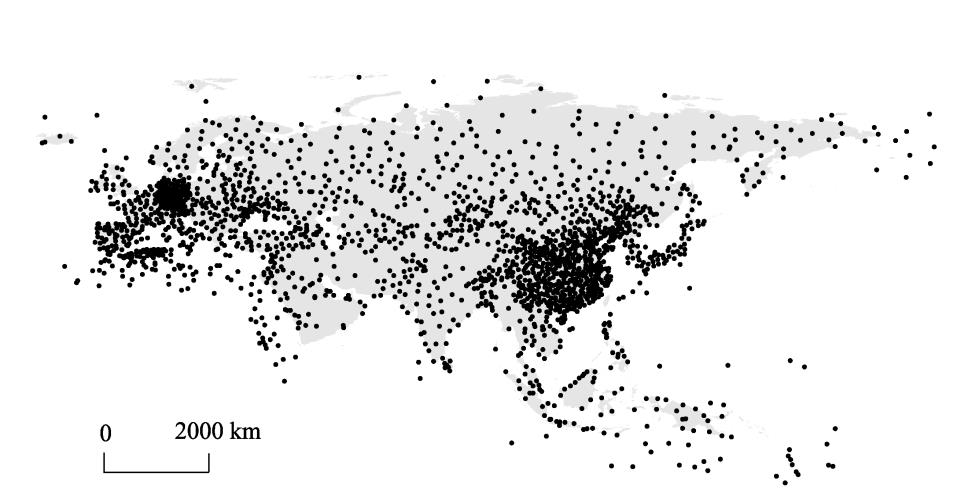
The basic datasets include the observation climatic data, climatic scenarios data and land cover data. The observation monthly climatic data has been collected from 2127 weather observation stations in Eurasia during 1981-2010 (Figure 1). The climatic scenario data of CMIP5 RCP26, RCP45 and RCP85 scenarios has been got from IPCC website during 2011-2100, and the land cover current data of Eurasia in 2010 has been downloaded from ftp://vct.geog.umd.edu/ST/ (Zhang et al., 2016). The mean annual biotemperature, average total annual precipitation and potential evapotranspiration ratio at a spatial resolution of 0.125° × 0.125° were respectively obtained by operating a high accuracy and speed method of surfacing modeling (HASM) (Yue, 2010, Yue et al., 2016) during all the four periods 1981 to 2010 (T0), 2011 to 2040 (T1), 2041 to 2070 (T2), and 2071 to 2100 (T3).

The spatial data of biome types at a spatial resolution of 0.125º × 0.125º in T0, T1, T2 and T3 were respectively generated by running the improved Holdridge life zone model, in terms of the spatial data of mean annual biotemperature (MAB), average total annual precipitation (TAP), and potential evapotranspiration ratio (PER) simulated by HASM (Yue et al., 2011; Fan et al., 2015). The HLZ model (Holdridge 1947, 1967, 1971) is a scheme which utilizes the three bioclimatic variables to formulate the biome distribution (Zhang, 1993; Yue et al., 2005, 2006). The HLZ types in Eurasia include Polar/Nival area, Subpolar/Alpine dry tundra, Subpolar/Alpine moist tundra, Subpolar/Alpine wet tundra, Subpolar/Alpine rain tundra, Cold temperate dry scrub, Cold temperate moist forest, Cold temperate wet forest, Cold temperate rain forest, Cool temperate scrub, Cool temperate steppe, Cool temperate moist forest, Cool temperate wet forest, Cool temperate rain forest, Warm temperate desert scrub, Warm temperate thorn steppe, Warm temperate dry forest, Warm temperate moist forest, Warm temperate wet forest, Subtropical desert scrub, Subtropical thorn woodland, Subtropical dry forest, Subtropical moist forest, Subtropical wet forest, Subtropical rain forest, Tropical desert scrub, Tropical thorn woodland, Tropical very dry forest, Tropical dry forest, Tropical moist forest, Tropical wet forest, Tropical rain forest, and Desert (Table 1).

The land cover data of Eurasia have been separated from the land cover data at a spatial resolution of 0.125° × 0.125° of the global rest in 2010. The land cover types were classified into 13 types by combining the land cover classification systems of FAO and UNEP (Gregorio and Jansen, 2001), IGBP, USGS, ESA GlobCover, and UMD, which include Evergreen broadleaf forest, Deciduous broadleaf forest, Evergreen needleleaf forest, Deciduous needleleaf forest, Mixed forest, Shrub land, Grasslands, Wetlands, Croplands, Water bodies, Snow and Ice, Built-up land, Barren or sparsely vegetated land (Table 1).

Land cover change is a complex process driven by natural factors, climate conditions, and human factors. If the impact of various factors is to be considered in the process of simulated predictive analysis, the entire study will become extremely complicated and it is impossible to start. Climate conditions such as mean annual biotemperature, average total annual precipitation and potential evapotranspiration ratio have directly impact on the natural course of land cover (Lauenroth et al., 1993). After comparing the corresponding relationship of the spatial distribution between biome types and land cover types, the distribution of HLZ types and land cover types are very similar on spatial pattern (Fan et al., 2005; Yue et al., 2007, 2011) (Figure 2). Therefore, SMLCS, as a grid-oriented, spatial explicit land cover scenarios model, has been improved to simulate land cover changes of Eurasia in 2040, 2070 and 2100.

In this paper, the land cover types has been replaced by the relative cover of each land cover type in every cell, e.g. a grid cell includes three land cover types which respectively contain 60% cropland, 25% forest land and 15% grassland, then the land cover data would consist of three probability data belonging to three different kinds of land cover types. That is to say, the new transition probability matrix can quantitatively describe the land cover spatial distribution characteristics within each HLZ type (Fan et al., 2015). Therefore, land cover type at a grid during next period would tend to the direction that the HLZ type appeared at the grid during next period, e.g. at grid (x, y), if probability of land cover type k corresponding to HLZ type occurred in t + 1 period is more than that corresponding to HLZ type occurred in t period, the cover probability of land cover type k at the grid would increase. Thus, when we create new probability formulation which indicates the probability of a grid cell to be covered by a certain land cover type, we have to take account the probability change of each land cover type corresponding to HLZ type between the former and next period. The new probability formulation and decision rules can be formulated as:

where x, y is the coordinate of grid cell; k is the type code of land cover; t is the variable of time; HLZP(x,y)k,trepresents the transition probability between land cover type k and the HLZ type appeared at grid (x, y) in t year. LP(x,y)k,tis the percentage of land cover type k contained in grid (x, y) which should satisfy the formula ∑k=122LP(x,y)k,t=1;LP(x,y)k,t+1is the transition probability of land cover type k in t+1 period; LC(x,y)t+1is the type value of land cover at grid (x, y) in t+1 period.

The major steps of the improved SMLCS include: 1) simulating the MAB, TAP and PER data in Eurasia by operating the HASM and simulating the HLZ types distribution by running the HLZ model; 2) establishing the transition probability matrix (Table 1) between HLZ types and land cover types by combining the HLZ type data during 1981-2010 on an average (Figure 2a) and the land cover data in 2010 (Figure 2b); 3) recognizing whether the HLZ type at grid cell (x, y) will change or not from t period to t+1 period; 4) assigning the grid cell (x, y) at t+1 period on the basis of the max value of transition probability; and 5) repeating step 3 and step 4 until all the grid cells of land cover type have been allocated at t+1 period.

The simulation results of land cover (Figures 3-5) under the RCP26, RCP45 and RCP85 scenarios show that the spatial distribution of land cover scenario would have a very similar regional change characteristic on the spatial pattern in Eurasia during 2010-2100. There would be a great difference in spatial distribution of forest and shrub because of the complicated terrain characteristics and heterogeneous climate change in Eurasia. Evergreen broadleaf forest would be mostly distributed in Southeast Asia. Evergreen needleleaf forest would mainly be distributed in Nordic Europe, East European Plain, Western Siberian Plain, Japan, South Korea, and hilly areas in South China. Deciduous needleleaf forest would be mainly distributed in Central Siberian Highlands and Eastern Siberia, which would cover about half of Russia’s area. Shrub land would be mainly distributed in the north and east of Russia, southwest China, northeast Laos, the border zone between India and Myanmar and the border zone between India and Pakistan, the north of United Kingdom, the south of Greece, most of Turkey, east of Georgia, and central Azerbaijan.

Grasslands would mainly be distributed in Tianshan Mountains, Tibetan Plateau, Inner Mongolian Plateau, Loess Plateau, Altai Mountains and areas around Tarim Basin of China, North Siberian Plain, Norway, the northwest of Iran, the north of Kazakhstan and the middle of Mongolia.

Croplands would mainly be distributed in the East European and Central European Plains. Croplands would mainly be distributed in Northeast China Plain, North China Plain, middle and lower reaches of the Yangtze River, Sichuan Basin and Guanzhong Basin of China. Hexi Corridor and the river alluvial sectors of Tianshan Mountains in China also would have relatively concentrated cultivated land. The centre of South Asia is one of the greatest alluvial plains in the world, which is formed by Indus, Ganges and Brahmaputra rivers, with dense river networks, numerous irrigation channels, and developed agriculture, such as India. In addi-tion, croplands would be mainly distributed in Thailand, Myanmar, Vietnam in IndoChinese Peninsula, the coastal area of Malay Archipelago.

Barren or sparsely vegetated land would mainly be distributed in Uzbekistan, Turkmenistan and southern Kazakhstan of Central Asia, and Iran, Saudi Arabia, Yemen of Western Asia. Moreover, barren or sparsely vegetated land would be distributed in southern Mongolia and Northwest China. In China, barren or sparsely vegetated land would mainly be distributed in the arid and desert areas in the northwest, namely Gurbantunggut Desert in Junggar Basin, Taklimakan Desert in Tarim Basin, the center of Qaidam Basin, and Tengger Desert, Alax Plateau.

Water bodies include rivers and lakes. The main water body area is river area, which include Volga River, Yenisei, Ob River, Ural River, Syr Darya, Tigris River, Euphrates River, Po, and Mekong. Lakes would mainly be distributed in Finland, named Country of Thousand Lakes that mainly include Baikal, and Aral Sea. In China, the river system mainly originates from Qilian and Hengduan mountains in the east of the Qinghai-Tibet Plateau, the mountainous areas around the Sichuan Basin, the Changbai Mountains in the northeast, the Greater Xinggan Mountains, and the hilly regions in South China. The distribution of water bodies would be more dispersed than other land cover types. Wetlands would mainly be distributed in Western Siberian Plain.

Snow and ice would mainly be distributed in the Himalayas, the high latitude zone in Nordic Europe and North Asia. Built-up land would mainly be distributed in areas that would be close to rivers, sufficient water resources, convenient to transport, fertile land and rich products, due to the formation and development factors of urban and the land use characteristics of artificial land.

During 2010-2100, the area of evergreen broadleaf forest, grasslands, croplands, water bodies and built-up land would increase while the areas of deciduous needleleaf forest and snow and ice would decrease under all three scenarios of RCP26, RCP45 and RCP85 (Tables 2-4) in all the three periods. The area of deciduous broadleaf forest would increase in all the three periods under all the scenarios except a decrease during 2010-2040 under the RCP26 scenario. The area of mixed forest and shrub land would decrease in all the three periods under the RCP26 scenario, which would increase during 2070-2100 under the two scenarios of RCP45 and RCP 85. Compared with 2010, the area of deciduous broadleaf forest, mixed forest, shrub land and wetlands would decrease in 2100 under all three scenarios. The area of wetlands would increase during 2010-2040 and then decrease during 2040-2100 under the two scenarios of RCP45 and RCP85, but which would increase from 2010 to 2070 and then decrease from 2070 to 2100 under the RCP26 scenario. The area of evergreen needleleaf forest would decrease during 2010-2070 and increase during 2070-2100 under the two scenarios of RCP26 and RCP45. But under the RCP85 scenario, the area of evergreen needleleaf forest would decrease during 2010-2040 and then increase during 2040-2100.

The area of barren or sparsely vegetated land would decrease during 2010-2040 and then increase during 2040-2100 under the two scenarios of RCP45 and RCP85, but it would decrease during 2010-2070 and then increase during 2070-2100 under the RCP 26 scenario.

In terms of the simulated results of land cover under the three scenarios of RCP26, RCP45 and RCP85 (Tables 2-7), most land cover types would generally have similar changing trends in the future, but which have some difference in different periods.

During 2010-2040: shrub land would have the greatest decrease area, down respectively by 187,409 km² and 146,044 km² under the two scenarios of RCP26 and RCP45, and evergreen needleleaf forest would have the greatest decrease area, down by 154,486 km² under the scenario RCP85; snow and ice would have the largest decrease rate, down respectively by 7.55% and 7.65% under the two scenarios of RCP26 and RCP45, and mixed forest would have the largest decrease rate, down by 9.50% under the scenario of RCP85; croplands would all have the greatest increase area, up by 318,257 km², 282,168 km² and 261,486 km², respectively, and wetlands would all have the largest increase rate, up by 6.56%, 6.98% and 7.31% under the three scenarios of RCP26, RCP45 and RCP85, respectively.

During 2040-2070: deciduous needleleaf forest would all have the greatest decrease area, down respectively by 150,898 km², 258,320 km² and 378,194 km², snow and ice would all have the largest decrease rate, down respectively by 10.42%, 10.65% and 19.72%, and water bodies would all have the largest increase rate, up by 4.35%, 7.34% and 11.61% under the three scenarios of RCP26, RCP45 and RCP85, respectively; croplands would have the greatest increase area, up by 147,521 km² and 170,314 km² under the two scenarios of RCP26 and RCP45, respectively; grasslands would have the greatest increase area that would be 194,795 km² un der the scenario RCP85.

During 2070-2080: under the three scenarios of RCP26, RCP45 and RCP85, deciduous needleleaf forest would all have the greatest decrease area, down respectively by 266,129 km², 876,051 km² and 1,172,782 km²; snow and ice would all have the largest decrease rate, down respectively by 9.55%, 25.86% and 26.73%; grasslands would all have the greatest increase area, up respectively by 105,312 km², 273,515 km² and 358,567 km²; water bodies would all have the largest increase rate, up respectively by 6.01%, 15.95% and 18.83%.

During 2010-2100, deciduous needleleaf forest would all have the greatest decrease area, down by 497,646 km², 1,160,752 km² and 1,563,850 km², respectively. Snow and ice would all have the largest decrease rate, being 25.09%, 38.82% and 45.51%, respectively. Croplands would all have the greatest increase area, up by 522,127 km², 545,765 km² and 575,733 km², respectively. Water bodies would all have the largest increase rate, being 14.44%, 28.29% and 38.08%, respectively.

The simulated results of land cover under the three scenarios RCP26, RCP45 and RCP85 indicate that deciduous needleleaf forest, mixed forest, shrub land, wetlands and snow and ice would generally decrease in Eurasia during 2010-2100. Snow and ice would have the fastest decreasing rate that would decrease by 36.44% on average. Shrub land would have the slowest decreasing rate that would decrease by 5.19% on average. Water bodies would have the fastest increasing rate that would increase by 26.94% on average. Barren or sparsely vegetated land would have the slowest increasing rate that would increase by 0.70%. Further more, the simulation results show that there would generally appear a similar change pattern of land cover driven by different levels of climate change scenarios in Eurasia. Land cover under the RCP85 scenario would generally have the fastest change rate, especially that the reducing trend of snow and ice would be much faster than that of scenarios of RC26 and RC45. There would have the lowest change rate of land cover in the scenario RCP26. The simulated results can approve proofs that climate change would directly impact on land cover change in Eurasia. For instance, the RCP85 is a highly energy-intensive scenario as a result of high population growth, a lower rate of technology development and non-climate policy, which represent a high scenario in climate change. Under the RC85 scenario, the temperature and precipitation would have the faster increase rate than other two scenarios of RCP26 and RCP45, so that there would have the largest change rate of land cover simulated by using the climatic data of the scenario RCP85. With the rapid increase of temperature and precipitation, the snow and ice would have a fast melting trend, the grasslands would also show an increasing trend, and the succession would occur between different forest types.

HLZ model can simulate long-term biome types, so SMLCS can also be used to simulate land cover types at long-term scale (Fan et al., 2013, 2015). In this paper, the aim of improved SMLCS is that can be used to simulate land cover change from the perspective of climate change because there is not enough socioeconomic data and human activities data in Eurasia. However, with the advance of the Belt and Road initiative, we believe that lots of socioeconomic data and human activities data would can be collected from more data sources, so in our future work, more parameter data will be considered into the next improved SMLCS which would include the agricultural pattern, population density, road construction, and government policy, etc. That is to say, we will focus on analyzing and discussing what is the coupling effect of climate change and human activities on land cover change, and then further improve the SMLCS.

Moreover, with the driving force and influence of climate change and human activities, the spatiotemporal distribution pattern of land cover in Eurasia has obviously changed since the beginning of the 21st century. How to understand and explain the land cover change is an important issue in the implementation of the Belt and Road Initiative. The current simulation results can reflect the land cover change scenarios driven by climate change, and can also provide the land cover data for the study of hydrological cycle, soil erosion and biological diversity in the context of climate change in Eurasia. We believed that further simulated results by operating the future improved SMLCS combined with human activities and policy factors will approve the more important data for supporting a series of major projects about the Belt and Road Initiative.

References

[1] M Adams R, A Fleming R, C Chang C et al. A reassessment of the economic effects of global climate change on U.S. agriculture. Climatic Change, 30, 147-167(1995).
[2] J Alcamo, J Kreileman G J, S Krol M et al. Modeling the global society-biosphere-climate system: Part 1: Model description and testing. Water Air & Soil Pollution, 76, 1-35(1994).
[3] Q Bai W, M Zhang Y, Z Yan J. Simulation of land use dynamics in the upper reaches of the Dadu River. Geographical Research, 24, 206-212(2005).
[4] K Clarke, S Hoppen, L Gaydos. A self-modifying cellular automaton model of historical urbanization in the San Francisco Bay area. Environment & Planning B Planning & Design, 24, 247-261(1997).
[5] M Fan Z, Y Li J, X Yue T. Land-cover changes of biome transition zones in Loess Plateau of China. Ecological Modelling, 252, 129-140(2013).
[6] M Fan Z, Y Li J, X Yue T et al. Scenarios of land cover in karst area of southwestern China. Environmental Earth Sciences, 74, 6407-6420(2015).
[7] M Fan Z, X Yue T, Y Liu J et al. Spatial and temporal distribution of land cover scenarios in China. Acta Geographica Sinica, 60, 941-952(2005).
[8] M Fan Z, X Zhang, Li Jing et al. Land-cover changes of national nature reserves in China. Journal of Geographical Sciences, 23, 258-270(2013).
[9] G Fischer, M Ermoliev Y, A Keyzer M et al. Simulating the socio-economic and biogeographical driving forces of land-use and land cover change: The IIASA land-use change model. IIASA Working Paper, WP-96-010.(1996).
[10] Q Gao Z, W Yi. Land use change in China and analysis of its driving forces using CLUE-S and Dinamica EGO model. Chinese Society of Agricultural Engineering, 28, 208-216(2012).
[11] D Gregorio A, M Jansen L J. Land cover classification system (LCCS): Classification concepts and user manual for software version 1.0. FAO.(2001).
[12] F Guo Y, B Yu X, G Jiang L et al. Scenarios analysis of land use change based on CLUE model in Jiangxi Province by 2030. Geographical Research, 31, 1016-1028(2012).
[13] Y He C, J Chen, J Shi P et al. Study on the spatial dynamic city model based on CA (Cellular Automata) model. Progress in Geography, 21, 188-119(2002).
[14] R Holdridge L. Determination of world plant formations from simple climate data. Science, 105, 367(1947).
[15] R Holdridge L. Life Zone Ecology. Libros Y. Materiales Educativos.(1967).
[16] R Holdridge L, C Grenke W, W H Hatheway et al. Forest Environments in Tropical Life Zones.(1971).
[17] T Ichinose, K Otsubo. Temporal structure of land use change in Asia. Journal of Global Environment Engineering, 9, 41-51(2003).
[18] K Lauenroth W, L Urban D, P Coffin D et al. Modeling vegetation structure-ecosystem process interactions across sites and ecosystems. Ecological Modelling, 67, 49-80(1993).
[19] J Li, M Fan Z, X Yue T. Spatio-temporal simulation of land cover scenarios in southwestern of China. Acta Ecologica Sinica, 34, 3266-3275(2014).
[20] X Li, L Yu, T Sohl et al. A cellular automata downscaling based 1 km global land use datasets (2010-2100). Science Bulletin, 61, 1651-1661(2016).
[21] I Turner B L, L Skole D, S Sanderson et al. Land-use and land-cover change, Science/research plan. Global Change Report, 43, 669-679(1995).
[22] A Veldkamp, O Fresco L. CLUE: A conceptual model to study the conversion of land use and its effects. Ecological Modelling, 85, 253-270(1996).
[23] H Verburg P. Exploring the spatial and temporal dynamics of land use with special reference to China. Wageningen University.(2000).
[24] H Verburg P, P Schot P, J Dijst M et al. Land use change modeling: Current practice and research priorities. GeoJournal, 61, 309-324(2004).
[25] H Verburg P, W Soepboer, A Veldkamp et al. Modeling the spatial dynamics of regional land use: The CLUE-S Model. Environmental Management, 30, 391-405(2002).
[26] H Verburg P, A Veldkamp, O Fresco L. Simulation of changes in the spatial pattern of land use in China. Applied Geography, 19, 211-233(1999).
[27] V Vuuren D P, J Edmonds, M Kainuma et al. The representative concentration pathways: An overview. Climatic Change, 109, 5(2011).
[28] F Wu. Calibration of stochastic cellular automata: The application to rural-urban land conversions. International Journal of Geographical Information Systems, 16, 795-818(2002).
[29] F Wu, J Webster C. Simulation of land development through the integration of cellular automata and multicriteria evaluation. Environment & Planning B Planning & Design, 25, 103-126(1998).
[30] X Yue T. 2010..
[31] T Yue, Z Fan, C Chen et al. Surface modelling of global terrestrial ecosystems under three climate change scenarios. Ecological Modelling, 222, 2342-2361(2011).
[32] X Yue T, M Fan Z, Y Liu J. Changes of major terrestrial ecosystems in China since 1960. Global and Planetary Change, 48, 287-302(2005).
[33] X Yue T, M Fan Z, Y Liu J et al. Scenarios of major terrestrial ecosystems in China. Ecological Modelling, 199, 363-376(2006).
[34] X Yue T, M Fan Z, Y Liu J. Scenarios of land cover in China. Global and Planetary Change, 55, 317-342(2007).
[35] X Yue T, A Wang Y, Y Liu J et al. Surface modelling of human population distribution in China. Ecological Modelling, 181, 461-478(2005).
[36] X Yue T, N Zhao, R Douglas Ramsey et al. Climate change trend in China, with improved accuracy. Climatic Change, 120, 137-151(2013).
[37] X Yue T, N Zhao, M Fan Z et al. CMIP5 downscaling and its uncertainty in China. Global and Planetary Change, 146, 30-37(2016).
[38] X Yue T, N Zhao, H Yang et al. A multi-grid method of high accuracy surface modeling and its validation. Transaction in GIS, 17, 943-952(2013).
[39] R Zhang, Q Huang C, X Zhan et al. Development and validation of the global surface type data product from S-NPP VIIRS. Remote Sensing Letters, 7, 51-60(2016).
[40] S Zhang X. A vegetation-climate classification system for global change studies in China. Quaternary Sciences, 13, 157-169(1993).
Set citation alerts for the article
Please enter your email address
© Copyright 2018-2021 | Chinese Laser Press. All Rights Reserved 沪ICP备15018463号-20