
Yunning Lu, Zeyang Liao, Fu-Li Li, Xue-Hua Wang, "Integrable high-efficiency generation of three-photon entangled states by a single incident photon," Photonics Res. 10, 389 (2022)
- Photonics Research
- Vol. 10, Issue 2, 389 (2022)
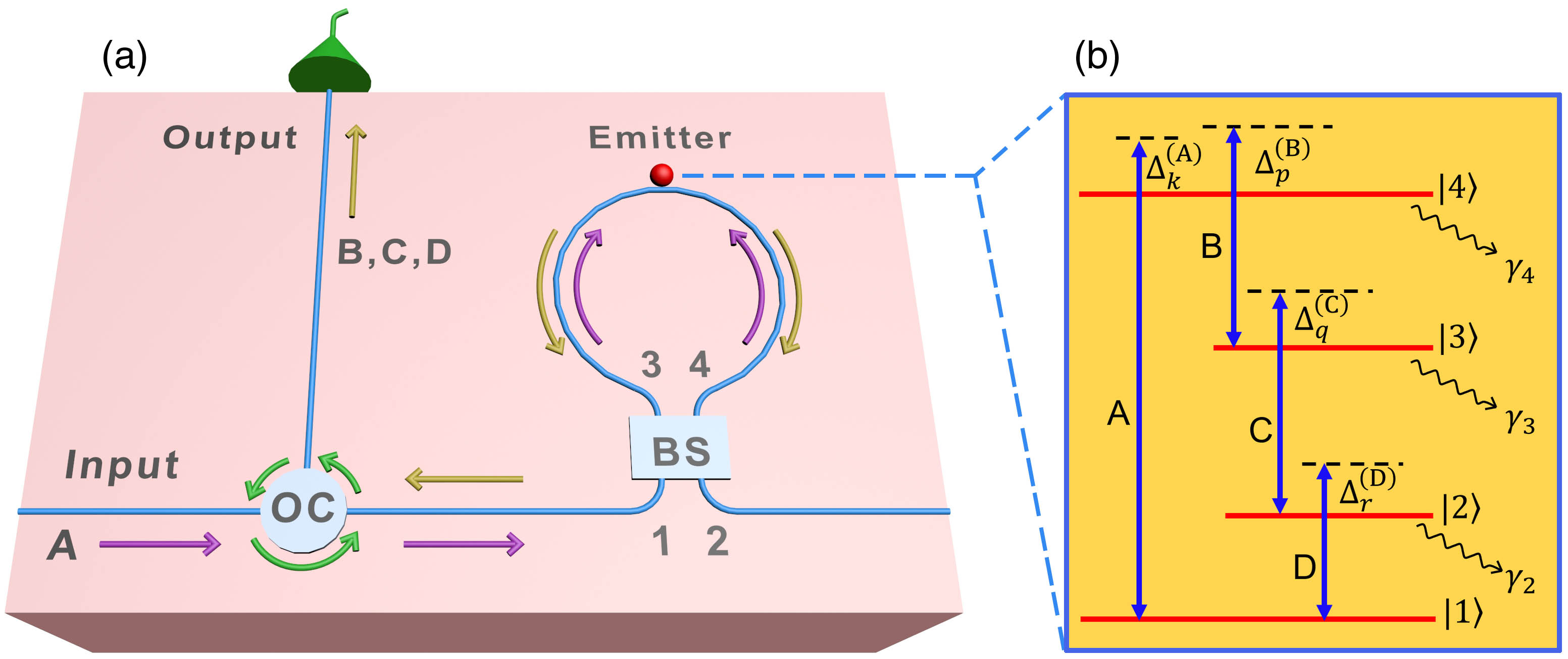
Fig. 1. Schematic of the system. (a) A Sagnac interferometer is a waveguide loop coupled to two external linear waveguides via a 50/50 beam splitter BS. An emitter is coupled to the waveguide loop. An optical circulator OC is used to distinguish the input and output photons. (b) Energy levels of the quantum emitter. Photons A, B, C, D are coupled to four transition paths of the emitter.
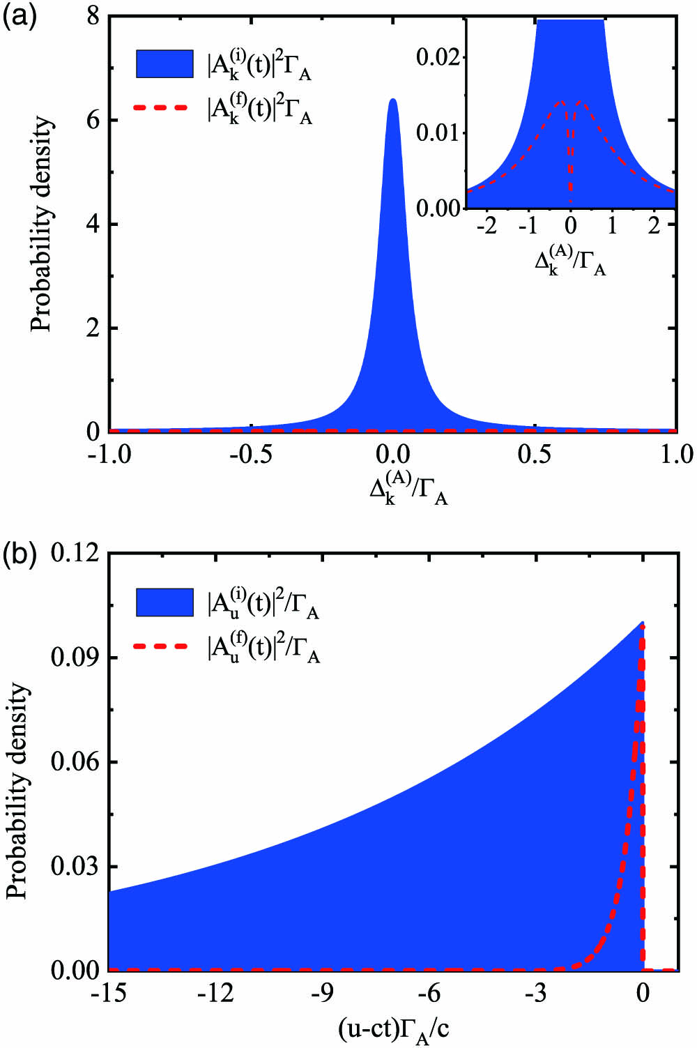
Fig. 2. (a) Frequency-space probability densities of photon A before and after scattering, | A k ( i ) ( t ) | 2 | A k ( f ) ( t ) | 2 | A k ( i ) ( t ) | 2 = 0 | A k ( f ) ( t ) | 2 = 0 | A u ( i ) ( t ) | 2 | A u ( f ) ( t ) | 2 Γ A = Γ B = Γ C = Γ D γ 4 = 0.02 Γ A δ A = 0 ϵ A = 0.05 Γ A
Fig. 3. (a) Real-space joint probability density | D x y z ( f ) ( t ) | 2 ( x − c t ) Γ A / c = − 2 | D x y z ( f ) ( t ) | 2 Γ B = Γ A Γ C = 1.2 Γ A Γ D = 0.5 Γ A γ 2 = γ 3 = γ 4 = 0.02 Γ A δ A = 0 ϵ A = 0.05 Γ A
Fig. 4. Frequency-space joint probability density of the three-photon state | D p q r ( f ) ( t ) | 2 ϵ A = 0.05 Γ A ϵ A = 0.1 Γ A Γ A = Γ B = Γ C = Γ D γ 2 = γ 3 = γ 4 = 0.02 Γ A δ A = 0
Fig. 5. (a) Entanglement entropy S 1 K 1 S 2 K 2 Γ C / Γ A ϵ A ϵ A = 0.05 Γ A ϵ A = 0.1 Γ A λ n ( 1 ) λ n ( 2 ) Γ C / Γ A = 1.5 ϵ A = 0.05 Γ A ϵ A = 0.1 Γ A Γ B = Γ D = Γ A γ 2 = γ 3 = γ 4 = 0.02 Γ A
Fig. 6. Probability of (a) three-photon state P BCD P A P Dis ϵ A Γ B P BCD P A Γ B / Γ A P BCD P A P Dis Γ B ϵ A / Γ A = 10 − 4 Γ C = Γ D = Γ A γ 2 = γ 3 = γ 4 = 0.02 Γ A δ A = 0
Fig. 7. (a) Entanglement entropy S 2 K 2 Γ D / Γ A ϵ A ϵ A = 0.05 Γ A ϵ A = 0.1 Γ A λ n ( 2 ) Γ D / Γ A = 1.5 ϵ A = 0.05 Γ A ϵ A = 0.1 Γ A Γ B = Γ C = Γ A γ 2 = γ 3 = γ 4 = 0.02 Γ A


Set citation alerts for the article
Please enter your email address

© Copyright 2018-2021 | Chinese Laser Press. All Rights Reserved 沪ICP备15018463号-20