• Photonics Research
  • Vol. 10, Issue 2, 389 (2022)
Yunning Lu1、2, Zeyang Liao1、3、*, Fu-Li Li2, and Xue-Hua Wang1、4、*
Author Affiliations
  • 1State Key Laboratory of Optoelectronic Materials and Technologies, School of Physics, Sun Yat-sen University, Guangzhou 510275, China
  • 2Shaanxi Province Key Laboratory of Quantum Information and Quantum Optoelectronic Devices, School of Physics, Xi’an Jiaotong University, Xi’an 710049, China
  • 3e-mail: liaozy7@mail.sysu.edu.cn
  • 4e-mail: wangxueh@mail.sysu.edu.cn
  • show less
    DOI: 10.1364/PRJ.443245 Cite this Article Set citation alerts
    Yunning Lu, Zeyang Liao, Fu-Li Li, Xue-Hua Wang. Integrable high-efficiency generation of three-photon entangled states by a single incident photon[J]. Photonics Research, 2022, 10(2): 389 Copy Citation Text show less

    Abstract

    Generation of multi-photon entangled states with high efficiency in integrated photonic quantum systems is still a big challenge. The usual three-photon generation efficiency based on the third-order nonlinear effect is extremely low. Here, we propose a scheme to generate three-photon correlated states, which are entangled states in frequency space and bound states in real space, with high efficiency. This method relies on two crucial processes. On one hand, by employing a Sagnac interferometer, an incident photon can be transformed into a symmetric superposition of the clockwise and counterclockwise modes of the Sagnac loop, which can then be perfectly absorbed by the emitter. On the other hand, the coupling strengths of the two transition paths of the emitter to the Sagnac loop are set to be equal, under which the absorbed photon can be emitted completely from the cascaded transition path due to quantum interference. By adjusting the coupling strengths among the three transition paths of the emitter and the waveguide modes, we can control the spectral entanglement and spatial separation among the three photons. Our proposal can be used to generate three-photon entangled states on demand, and the efficiency can be higher than 90% with some practical parameters, which can find important applications in integrated quantum information processing.

    1. INTRODUCTION

    Quantum entanglement, “spooky action at a distance,” is one of the most intriguing phenomena in quantum mechanics. The generation of entangled photon states plays a crucial role in quantum information, quantum computation, and quantum metrology [17]. Two-photon entangled states, the simplest multi-photon entangled states, can be prepared based on second-order parametric downconversion in nonlinear media [815], but the generation efficiency is usually very low. For example, in beta-barium borate crystals, only one in every 1012 pumped photons can be transformed into a two-photon state. The efficiency can be significantly improved by embedding semiconductor quantum dots in broadband photonic nanostructures [16], and the quantum states of a single photon can be on-demand controlled [17,18]. In comparison to the two-photon entangled pair, the efficiency to generate three-photon entangled states is even lower because the third-order nonlinear coefficient χ(3) is usually extremely small, typically ranging from 1021  m2/V2 to 1019  m2/V2 [19]. For example, for the type-I process in TiO2, the effective cubic susceptibility is χ(3)=2.1×10²⁰  m2/V2. When a TiO2 crystal with a length of 5 mm is pumped by a continuous wave with power 100  mW (about 1017 photons per second), only a few three-photon states can be obtained per hour [20]. Generation of three-photon entangled states with high efficiency is still a big challenge.

    In addition to efficiency, integrability is another important property to be considered. Quantum advantages have been demonstrated in several experiments [2123]. The next ambition is to build a scalable error-correctable quantum information device in an integrated chip [24]. The usual way to produce multi-photon entangled states based on nonlinear crystals is difficult to be integrated into a chip. In recent years, waveguide–quantum electrodynamics (waveguide-QED) systems have been demonstrated as a promising platform to build a scalable and integrable quantum network [2530], which has been realized in several different physical systems such as quantum dots coupled with metallic nanowires [31,32], superconducting qubits coupled with one-dimensional (1D) open transmission lines [3340], trapped atoms coupled with photonic crystal waveguides [4146], and trapped cold atoms coupled with 1D nanofibers [4749]. Several schemes have been proposed to generate photon–photon correlation in the waveguide-QED system. When two or more independently propagating guided photons are scattered by an emitter, bound states of photons can be generated [5054]. When two distinguishable guided photons interact with the two different transition paths of a Ξ-type three-level emitter, the two output photons can be entangled in frequency space [55]. However, in the above works, multiple photons need to be incident, and the probability that the photons become entangled is usually less than 50% because the incident photons are unidirectional, which can be decomposed as an equal superposition of symmetric and antisymmetric modes, and only the symmetric mode can interact with the emitter. In addition, in these schemes, not all of the absorbed photons become correlated after scattering. Bradford et al. proposed a method for highly efficient single-photon frequency conversion using a Sagnac interferometer [56], and it was generalized to generate two entangled photons with high efficiency [57]. However, in that scheme, they used a Δtype emitter, which cannot be realized in the usual quantum system due to the forbidden selection rule of electric dipole transition.

    Here, we propose a scheme to deterministically generate three-photon entangled states by an incident single photon in an integrated waveguide-QED system. We employ a Sagnac interferometer, which is a waveguide loop coupled to two 1D line waveguides via a 50/50 beam splitter (BS), and an incident photon from a line waveguide can be transformed into a symmetric superposition of the clockwise and counterclockwise modes of the waveguide loop, which can then be completely absorbed by a four-level emitter coupled to the waveguide loop. When the coupling strengths of two transition paths of the emitter are equal, the absorbed photon energy can be emitted completely from the cascaded pathway due to the complete destructive interference between the directly transmitted photon amplitude and the absorbed, re-emitted photon amplitude. After scattering, the single incident photon can be transferred to three lower-frequency photons that are entangled in frequency and bound together in real space. By manipulating the coupling strengths among the three transition paths of the emitter and the waveguide modes, we can control the spectral entanglement and spatial binding among the three photons. In our proposal, the output time of the three-photon state is determined by the input time of the initial photon and thus can be generated on demand. Even if considering the effect of some nonideal factors, such as emitter dissipation and off-resonance components in the input photon pulse, the success probability of generating the three-photon state can still be more than 90%.

    This paper is arranged as follows. In Section 2, we introduce the model of our system. In Section 3, we calculate the three-photon state generated in our system, and discuss its spectral entanglement and spatial binding. In Section 4, we summarize our results.

    2. MODEL AND HAMILTONIAN

    The model we consider is shown in Fig. 1(a). A Sagnac interferometer [58] is a waveguide loop coupled to two external linear waveguides via a 50/50 BS. The BS has four ports, i.e., 1, 2, 3, and 4. Ports 1 and 2 are connected to the external waveguides, and ports 3 and 4 are connected to the waveguide loop. When a photon enters the waveguide loop from port 1 (2), it will become the symmetric (antisymmetric) superposition of the clockwise and counterclockwise modes of the loop. Conversely, a photon in the symmetric (antisymmetric) superposition of the clockwise and counterclockwise modes of the waveguide loop will leave the system from port 1 (2). A quantum emitter is strongly coupled to the waveguide loop at a position that is symmetrical with respect to the 50/50 BS, i.e., the position of the emitter has an equal optical path length to ports 3 and 4. Thus, the emitter is at an antinode of the symmetric mode photon, and at a node of the antisymmetric mode photon. The emitter can interact with the symmetric mode photon, and cannot interact with the antisymmetric mode photon. Here, the necessity of the use of the Sagnec interferometer should be emphasized. The Sagnac interferometer can transform a unidirectional photon into a symmetric superposition of the clockwise and counterclockwise modes of the waveguide loop. The symmetric-mode photon can interact with the emitter with a probability of 100%, and the probability of parametric downconversion may approach 100%. If we do not use a Sagnac interferometer, a unidirectional incident photon should be regarded as an equal superposition of symmetric and antisymmetric modes, and only the symmetric mode can interact with the emitter. The photon can be absorbed by the emitter with at most 50% probability, and therefore the probability of parametric downconversion is at most 50%. The Sagnac interferometer improves the probability significantly. On the left side of the system, an optical circulator (OC) is used to distinguish the input and output paths. The OC is a nonreciprocal optical device, and it allows photons to propagate along a special direction, but forbids photons to propagate along the opposite direction. For example, it is theoretically proposed [59,60] and experimentally demonstrated [61,62] that an OC can be a system in which a quantum emitter is chirally coupled to a whispering-gallery-mode microresonator, and the microresonator is coupled to two waveguides. The three ports of the two waveguides are the input and output ports of the OC. We assume that the waveguide loop in our model can support a continuum of photonic modes, and has an approximated linear dispersion relation ω=ck around the resonance transition frequency of the emitter.

    Schematic of the system. (a) A Sagnac interferometer is a waveguide loop coupled to two external linear waveguides via a 50/50 beam splitter BS. An emitter is coupled to the waveguide loop. An optical circulator OC is used to distinguish the input and output photons. (b) Energy levels of the quantum emitter. Photons A, B, C, D are coupled to four transition paths of the emitter.

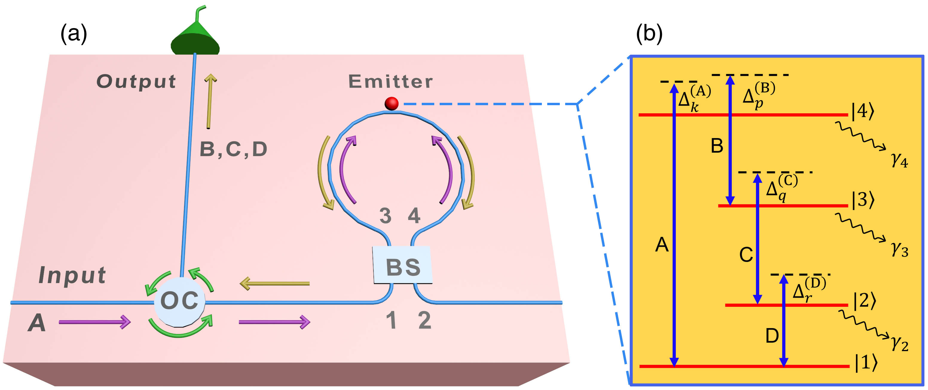
    Figure 1.Schematic of the system. (a) A Sagnac interferometer is a waveguide loop coupled to two external linear waveguides via a 50/50 beam splitter BS. An emitter is coupled to the waveguide loop. An optical circulator OC is used to distinguish the input and output photons. (b) Energy levels of the quantum emitter. Photons A, B, C, D are coupled to four transition paths of the emitter.

    The quantum emitter is assumed to be a four-level system with energy levels shown in Fig. 1(b). The four energy states are denoted as |1, |2, |3, and |4, with energies ω1, ω2, ω3, and ω4, respectively. Here, we have set =1 throughout this paper. We assume that the ground state |1 is a stable state, and the other three states can dissipate energy into free space at rates γ2, γ3, and γ4. An alkali atom such as rubidium is a possible candidate for the quantum emitter [63]. For example, the transition among the four energy levels |1|4|3|2|1 can be 5S6P6S5P5S. Four waveguide photon modes with different frequencies denoted as A, B, C, and D can be coupled to the four transition paths of the emitter, and their detunings are denoted as Δk(A), Δp(B), Δq(C), and Δr(D), respectively.

    We define an unperturbed Hamiltonian of the system: H0=ω1|11|+ω2|22|+ω3|33|+ω4|44|+n=e,o  f=a,b,c,ddkωffnkfnk,where ωa=ω4ω1, ωb=ω4ω3, ωc=ω3ω2, and ωd=ω2ω1 are the frequency spacings of the emitter energy levels. In the interaction picture, with respect to H0, the effective Hamiltonian of the system can be written as HI=HI(e)+HI(o). Here, HI(e) includes the energy of the even-mode photons, the effective Hamiltonian of the emitter including the dissipations, and their interaction: HI(e)=dk[Δk(A)aekaek+Δk(B)bekbek+Δk(C)cekcek+Δk(D)dekdek]iγ2/2|22|iγ3/2|33|iγ4/2|44|+f=a,b,c,ddk2Vf(σf+fek+fekσf),where σa+=|41|, σb+=|43|, σc+=|32|, and σd+=|21| are raising operators of the emitter, and σf is the Hermitian of σf+ (f=a,b,c,d). HI(o)=dk[Δk(A)aokaok+Δk(B)bokbok+Δk(C)cokcok+Δk(D)dokdok] is the Hamiltonian of the odd-mode photons.

    In the Hamiltonian, Va, Vb, Vc, and Vd are the coupling strengths between photons A, B, C, D and the corresponding transitions of the emitter, respectively. aek (aek), bek (bek), cek (cek), and dek (dek) are the creation (annihilation) operators of the even modes of photons A, B, C, and D, with wave vector k, respectively. They are defined as the symmetric superposition of the creation (annihilation) operators of the clockwise- and counterclockwise-propagation photon modes fek=(fcw,k+fccw,k)/2, fek=(fcw,k+fccw,k)/2, with f=a,b,c,d. Likely, aok (aok), bok (bok), cok (cok), and dok (dok) are the creation (annihilation) operators of the odd modes of photons A, B, C, and D, with wave vector k, respectively. They are defined as the antisymmetric superposition of the creation (annihilation) operators of the clockwise- and counter clockwise-propagation photon modes fok=(fcw,kfccw,k)/2, fok=(fcw,kfccw,k)2, with f=a,b,c,d. It is clearly seen that only even-mode photons interact with the emitter, and odd-mode photons do not interact with the emitter. The even-mode Hamiltonian (2) is used for calculations in the following section.

    3. GENERATION OF THREE-PHOTON CORRELATED STATES

    In this section, we consider the scattering properties of a single photon wave packet by a four-level emitter coupled to a waveguide loop. We first derive a general analytical expression for the output states in the first subsection. Then we analyze the real space properties of the output state. In the third subsection, we study the spectral entanglement properties of the output three-photon state.

    A. General Dynamics of the System

    The quantum emitter is assumed to be in state |1 initially. A single photon pulse denoted as A with frequency near resonance to the transition |1|4 is incident from port “Input.” This photon then passes through the 50/50 BS and enters the waveguide loop. Since this photon enters the waveguide loop from port 1, it is in a symmetric superposition of the clockwise and counter-clockwise propagating modes in the waveguide loop.

    Before scattering, photon A is given by |Ψ(i)(t)=dkAk(i)(t)aek|Ø,1,where Ak(0) is its amplitude in momentum space with wave vector k. For perfect excitation, the photon is assumed to have a Lorentzian spectrum given by Ak(i)(t)=ϵAπ1Δk(A)δA+iϵA.

    Here, Δk(A) is the detuning between the k component of photon A and the emitter transition |1|4. δA is the detuning between the peak frequency of photon A and the frequency of the emitter transition |1|4. ϵA is the spectral width of photon A. In real space, the state of photon A is |Ψ(i)(t)=duAu(i)(t)ae(u)|Ø,1,where Au(i)(t)=i2ϵAexp[i(ωa+δAiϵA)(ctu)/c]θ(ctu).

    The corresponding probability density is given by |Au(i)(t)|2=2ϵAexp[2ϵA(ctu)/c]θ(ctu).

    When the scattering is finished (i.e., t1/ϵA, 1/ΓA, 1/ΓB, 1/ΓC, 1/ΓD), the state of the system is |Ψ(f)(t)=dkAk(f)(t)aek|Ø,1+dpBp(f)(t)bep|Ø,3+dpdqCpq(f)(t)bepceq|Ø,2+dpdqdrDpqr(f)(t)bepceqder|Ø,1+E(f)(t)|Ø,4,where Ak(f)(t)=ϵAπeiΔk(A)tΔk(A)δA+iϵA×Δk(A)+iγ4/2iΓA/2+iΓB/2Δk(A)+iΓ4/2,Dpqr(f)(t)=i2πϵAΓAΓBΓCΓDπeiΔpqr(BCD)t×1Δpqr(BCD)δA+iϵA1Δpqr(BCD)+iΓ4/2×1Δqr(CD)+iΓ3/21Δr(D)+iΓ2/2,and Bp(f)(t)=Cpq(f)(t)=E(f)(t)=0. Here, Δpqr(BCD)=Δp(B)+Δq(C)+Δr(D), and Δqr(CD)=Δq(C)+Δr(D). Γ4=γ4+ΓA+ΓB, Γ3=γ3+ΓC, and Γ2=γ2+ΓD are the total emission rate of emitter energy levels |4, |3, and |2, respectively. ΓA=4πVa2, ΓB=4πVb2, ΓC=4πVc2, and ΓD=4πVd2 are spontaneous emission rates from the emitter to the waveguide modes through transition paths |4|1, |4|3, |3|2, and |2|1, respectively. Ak(f)(t) is the residual amplitude of photon A after scattering. Dpqr(f)(t) is the amplitude of the generated three-photon state. Bp(f)(t), Cpq(f)(t), and E(f)(t) are zero because the emitter cannot stay in excited state |4, |3, or |2 after scattering. This is the main result in this subsection. The derivation of state [Eq. (8)] is shown in Appendix A.

    Equation (9a) is the amplitude of photon A Ak(f)(t) after scattering. It results from the coherent superposition of two parts. The first part is the initial amplitude of the incident photon. The second part is the emission amplitude from the transition |4|1 during scattering. In Eq. (9a), it is shown that in an ideal situation (monochromatic wave with no detuning Δk(A)=0 and absence of dissipation γ4=0), when condition ΓA=ΓB is satisfied, we have Ak(f)(t)=0, which indicates that incident photon A can be absorbed completely. An intuitive and physical explanation is that when the emitter is pumped from ground state |1 into excited state |4 by incident photon A with a certain probability, under the condition ΓA=ΓB, the emitter may emit the amplitude of photon A through transition |4|1 and the amplitude of photon B through transition |4|3 with equal probability. The amplitude of photon A emitted through transition |4|1 and the initial amplitude of incident photon A are equal in modulus and opposite in phase, and interfere completely destructively. As a result, photon A is absorbed completely. At the same time, photon B is generated with probability 100% through transition |4|3 of the emitter. Then photons C and D are generated through transitions |3|2 and |2|1 successively. Thus, incident photon A is absorbed and three photons B, C, and D are generated with probability 100% in an ideal situation. In Fig. 2(a), according to Eqs. (4) and (9a), we show the frequency-space probability density of photon A before (|Ak(i)|2) and after (|Ak(f)(t)|2) scattering. Indeed, with some practical parameters, the resonant frequency component is completely absorbed, and the whole photon A with a finite spectrum width can be almost entirely absorbed [64,65].

    (a) Frequency-space probability densities of photon A before and after scattering, |Ak(i)(t)|2 and |Ak(f)(t)|2. The inset figure is the enlarged detail of the area around |Ak(i)(t)|2=0 and |Ak(f)(t)|2=0. (b) Real-space probability densities of photon A before and after scattering, |Au(i)(t)|2 and |Au(f)(t)|2. The parameters are ΓA=ΓB=ΓC=ΓD, γ4=0.02ΓA, δA=0, ϵA=0.05ΓA.

    Figure 2.(a) Frequency-space probability densities of photon A before and after scattering, |Ak(i)(t)|2 and |Ak(f)(t)|2. The inset figure is the enlarged detail of the area around |Ak(i)(t)|2=0 and |Ak(f)(t)|2=0. (b) Real-space probability densities of photon A before and after scattering, |Au(i)(t)|2 and |Au(f)(t)|2. The parameters are ΓA=ΓB=ΓC=ΓD, γ4=0.02ΓA, δA=0, ϵA=0.05ΓA.

    B. Three-Photon Bound State in Real Space

    We consider the spatial properties of the three-photon state generated in our scheme. We transform the photon state [Eq. (8)] in wave vector space into real space: |Ψ(f)(t)S=duAu(f)(t)ae(u)|Ø,1+dxdydzDxyz(f)(t)be(x)ce(y)de(z)|Ø,1,where Au(f)(t)=i2ϵAθ(ctu)×exp[i(ωa+δAiϵA)(ctu)/c]+i2ϵAexp[iωa(ctu)/c]θ(ctu)×{exp[(ϵA+iδA)(ctu)/c]exp[(Γ4/2)(ctu)/c]}×ΓA/(Γ4/2ϵAiδA),Dxyz(f)(t)=2ϵAΓAΓBΓCΓD×θ(ctx)θ(xy)θ(yz)×exp[iωb(ctx)/c]×exp[iωc(cty)/c]×exp[iωd(ctz)/c]×{exp[(ϵA+iδA)(ctx)/c]exp[(Γ4/2)(ctx)/c]}×[1/(δAiϵA+iΓ4/2)]×exp[(Γ3/2)(xy)/c]×exp[(Γ2/2)(yz)/c]are the real-space wave functions of photon A and generated B, C, D three-photon state. The derivation of Eq. (10) is shown in Appendix B.

    In Fig. 2(b), we plot the real-space probability densities of photon A before and after scattering according to Eqs. (7) and (11a), respectively. The area under the curve |Au(f)(t)|2 is much smaller than the area under the curve |Au(i)|2, which indicates that photon A is absorbed by the emitter with a high probability after scattering.

    In Fig. 3(a), we plot the real-space joint probability densities |Dxyz(f)(t)|2 of B, C, D three-photon states as functions of the separation xy between photons B and C, and the separation yz between photons C and D, according to Eq. (11b). We find |Dxyz(f)(t)|2 takes the maximum value when xy=0 and yz=0, and decreases to zero with the increasing of xy and yz. Thus, photons B, C, and D are in bound state in real space. In fact, when ΓC takes a bigger value, |Dxyz(f)(t)|2 decreases faster with the increasing of variable xy, and therefore photons B and C are more inclined to stay together. Similarly, when ΓD takes a bigger value, photons C and D are more likely to stay together. When both ΓC and ΓD are large, all three photons stay together with smaller separations. From the above discussion, it is clearly shown that a three-photon bound state is generated. The red dashed curve (blue dashed curve) shows that |Dxyz(f)(t)|2 decreases exponentially with the increasing of the separation xy of photons B and C (separation yz of photons C and D) when yz=0 (xy=0). Here, Γ3=ΓC+γ3, and Γ2=ΓD+γ2.

    (a) Real-space joint probability density |Dxyz(f)(t)|2 of B, C, D three-photon state. The parameter is (x−ct)ΓA/c=−2. (b) Real-space probability density of photons B, C, and D by integrating |Dxyz(f)(t)|2 over the position of photons C, D (B, D, or B, C). In both figures, other parameters are ΓB=ΓA, ΓC=1.2ΓA, ΓD=0.5ΓA, γ2=γ3=γ4=0.02ΓA, δA=0, ϵA=0.05ΓA.

    Figure 3.(a) Real-space joint probability density |Dxyz(f)(t)|2 of B, C, D three-photon state. The parameter is (xct)ΓA/c=2. (b) Real-space probability density of photons B, C, and D by integrating |Dxyz(f)(t)|2 over the position of photons C, D (B, D, or B, C). In both figures, other parameters are ΓB=ΓA, ΓC=1.2ΓA, ΓD=0.5ΓA, γ2=γ3=γ4=0.02ΓA, δA=0, ϵA=0.05ΓA.

    After integrating |Dxyz(f)(t)|2 over the position of photons C, D (photons B, D, or photons B, C), we show the real-space probability densities of photons B, C, and D in Fig. 3(b). We can see that photons B, C, and D propagate in 1D space, and appear successively in position w with increasing of time t. This is because the three photons were emitted successively through the cascaded transition path |4|3|2|1. In all three photon packets, the probability densities first increase rapidly, and then decrease nearly exponentially. The reason is that the initial incident photon is a packet decreasing exponentially, and when the head of the incident photon arrives and begins to excite the emitter, the population in excited states |4, |3, and |2 increases from zero to their maximum values rapidly, and then decreases nearly exponentially.

    C. Three-Photon Entangled State in Frequency Space

    In this subsection, we analyze the correlation properties of the generated three-photon state in frequency space. In Fig. 4, according to Eq. (9b), we show the frequency-space joint probability densities |Dpqr(f)(t)|2 of B, C, D three-photon state, as functions of detunings Δp(B), Δq(C), and Δr(D), with different incident photon A spectral widths ϵA. Since it is difficult to show the total three-dimensional frequency space in a two-dimensional plane, here, we choose the three cross sections to present the quantum correlation of the generated three-photon state, i.e., Δr(D)=0, Δq(C)=0, and Δp(B)=0. In Fig. 4(a), we have ϵA=0.05ΓA, and in Fig. 4(b), we have ϵA=0.1ΓA. It is clearly seen from Fig. 4 that |Dpqr(f)(t)|2 are mainly distributed along the lines Δp(B)+Δq(C)=0, Δp(B)+Δr(D)=0, and Δq(C)+Δr(D)=0. In fact, in the three-dimensional frequency space, |Dpqr(f)(t)|2 are mainly distributed around the area Δp(B)+Δq(C)+Δr(D)=0. This indicates that the frequencies of photons B, C, and D are entangled. This is because the total energy of photons B, C, and D should be equal to the energy of initial photon A, if the dissipations are not serious (γ2,γ3,γ4ΓA, ΓB,ΓC, ΓD). The energy conservation leads to the frequency entanglement of photons B, C, and D. Furthermore, by comparing Figs. 4(a) and 4(b), we can see that a narrower spectral width ϵA of incident photon A leads to thinner lines of |Dpqr(f)(t)|2, and therefore a stronger frequency entanglement among the three photons.

    Frequency-space joint probability density of the three-photon state |Dpqr(f)(t)|2. The parameters are (a) ϵA=0.05ΓA; (b) ϵA=0.1ΓA. Other parameters are ΓA=ΓB=ΓC=ΓD, γ2=γ3=γ4=0.02ΓA, δA=0.

    Figure 4.Frequency-space joint probability density of the three-photon state |Dpqr(f)(t)|2. The parameters are (a) ϵA=0.05ΓA; (b) ϵA=0.1ΓA. Other parameters are ΓA=ΓB=ΓC=ΓD, γ2=γ3=γ4=0.02ΓA, δA=0.

    To quantify the entanglement of the generated three-photon state, we first normalize the three-photon state as |ϕBCD(f)=dpdqdrDpqr(f)(t)PBCDbepceqder|Ø,1,where PBCD is the probability of generating the three-photon state. Then we decompose the three-photon state as two parts, and calculate the degree of entanglement between them. Here, we consider two different decompositions. In the first situation, photon B is treated as one part, and photons C and D are treated as the other part. In the second situation, photons B and C are one part, and photon D is the other part. For these two situations, we perform two kinds of Schmidt decompositions for the three-photon state as |ϕBCD(f)=nλn(1)|ϕB|ϕCD,|ϕBCD(f)=nλn(2)|ϕBC|ϕD,respectively. Here, {λn(1)} are the joint eigenvalues of the reduced density matrix of photon B and the reduced density matrix of the two-photon part C, D. {λn(1)} can be obtained by numerically calculating the eigenvalues of the reduced density matrix of photon B. In the numerical calculation of {λn(1)}, we first calculate the reduced density matrix of photon B by tracing over photons C and D ρB=TrCD(|ϕBCD(f)ϕBCD(f)|) analytically. The expression of ρB is given in Appendix C. We discretize the expression of ρB and transform it into a two-dimensional matrix with finite size. To obtain the eigenvalues with high enough precision, the values in every dimension of the matrix have a large enough value range, and small enough intervals. Then we obtain eigenvalues {λn(1)} of the matrix ρB by numerical calculation software. In principle, the reduced density matrix of photon B has infinite eigenvalues, but only a finite number of eigenvalues have nonnegligible values that need to be included in the calculation. Similarly, {λn(2)} are the joint eigenvalues of the reduced density matrix of the two-photon part B, C and the reduced density matrix of photon D, and they can be obtained by numerically calculating the eigenvalues of the reduced density matrix of photon D. We calculate the reduced density matrix of photon D by tracing over photons B and C ρD=TrBC(|ϕBCD(f)ϕBCD(f)|) analytically. The reduced density matrices of photon D are given in Appendix C. With the same method as calculating {λn(1)}, we can obtain the eigenvalues {λn(2)} of the reduced density matrices of photon D. With {λn(1)} and {λn(2)}, we can calculate the entropies of entanglement as S1=nλn(1)log2λn(1),S2=nλn(2)log2λn(2),and the Schmidt numbers K1=1nλn(1)2,K2=1nλn(2)2.

    We first discuss the entanglement between photon B and the two-photon part including C and D. In Figs. 5(a) and 5(b), we show the entropy of entanglement S1 and the Schmidt number K1 as functions of coupling strength ΓC, with different incident photon spectral widths ϵA. It is shown that as ΓC increases, both S1 and K1 increase, and therefore the entanglement increases. This is because after the emitter decays from state |4 to |3 by emitting photon B, a stronger coupling strength ΓC allows the emitter to decay from state |3 to |2 and |1 faster, and emit photons C and D faster. Therefore, photons B and C, D are more inclined to be bound together and have a higher degree of entanglement. We also find that a smaller incident photon band width ϵA leads to higher values of S1 and K1. In the inset in Fig. 5(b), we set ΓC=1.5ΓA, and show the first 25 joint eigenvalues λn(1), n=1,2,...,25. We can see that with a smaller ϵA, there are more effective eigenvalues, which results in a higher degree of entanglement. The reason is that a smaller incident photon bandwidth ϵA leads to a narrower joint spectrum bandwidth of the three-photon state due to the stronger restriction by the energy conversation law. Then we discuss the entanglement between two-photon part B, C and photon D. In Figs. 5(c) and 5(d), we show the entropy of entanglement S2 and the Schmidt number K2 as functions of coupling strength ΓC, with different incident photon spectral widths ϵA. We find that when ΓC/ΓA<1, i.e., ΓC<ΓD, as ΓC decreases, both S2 and K2 increase, and therefore the entanglement increases. This is because with a smaller ΓC, the emitter in |3 emits photon C more slowly and decays to |2, and then the emitter will emit photon D fast and decay to |1. Therefore, photons B, C, and D are more inclined to be bound together and have a higher degree of entanglement. When ΓC>ΓD, as ΓC increases, both S2 and K2 tend to be constants. The inset in Fig. 5(d) shows that a smaller ϵA leads to a higher degree of entanglement, which is similar to the inset in Fig. 5(b). We also have studied the effect of ΓD on S1, K1, S2, and K2. We find that the value of ΓD does not affect S1 and K1. The effect of ΓD on S2 and K2 is shown in Fig. 7 in Appendix C, which is similar to the effect of ΓC on S1 and K1 in Figs. 5(a) and 5(b).

    (a) Entanglement entropy S1 and (b) Schmidt number K1 of photon B and two-photon part C, D, (c) entanglement entropy S2 and (d) Schmidt number K2 of two-photon part B, C and photon D, as functions of ΓC/ΓA with different values of ϵA. In all figures, red curves with triangles: ϵA=0.05ΓA; blue curves with squares: ϵA=0.1ΓA. Insets in (b) and (d) show the first 25 joint eigenvalues {λn(1)} and {λn(2)} of the reduced density matrix of photon B and photon D with ΓC/ΓA=1.5, respectively. Red circles: ϵA=0.05ΓA; blue asterisks: ϵA=0.1ΓA. Other parameters are: ΓB=ΓD=ΓA, γ2=γ3=γ4=0.02ΓA.

    Figure 5.(a) Entanglement entropy S1 and (b) Schmidt number K1 of photon B and two-photon part C, D, (c) entanglement entropy S2 and (d) Schmidt number K2 of two-photon part B, C and photon D, as functions of ΓC/ΓA with different values of ϵA. In all figures, red curves with triangles: ϵA=0.05ΓA; blue curves with squares: ϵA=0.1ΓA. Insets in (b) and (d) show the first 25 joint eigenvalues {λn(1)} and {λn(2)} of the reduced density matrix of photon B and photon D with ΓC/ΓA=1.5, respectively. Red circles: ϵA=0.05ΓA; blue asterisks: ϵA=0.1ΓA. Other parameters are: ΓB=ΓD=ΓA, γ2=γ3=γ4=0.02ΓA.

    In Figs. 6(a)–6(c), we show the probability of generating B, C, D three-photon state PBCD, surviving A photon probability PA, and dissipation probability PDis, respectively, as functions of spectrum width ϵA of incident photon A and coupling strengths ΓB. The derivation of PBCD, PA, and PDis is shown in Appendix D. It is shown that smaller ϵA leads to higher PBCD [Fig. 6(a)] and lower PA [Fig. 6(b)]. This is because for smaller ϵA, incident photon A has more resonant components, and the efficiency of frequency downconversion is higher. We also find that around the area ΓB/ΓA=1, PBCD takes its maximum value and PA takes its minimum value, which means that incident photon A can be transformed into a three-photon state with maximum probability. This is because around the area ΓB/ΓA=1, the directly transmitted amplitude of incident photon A and the re-emitted amplitude of photon A destructively interfere, which results in the total absorption of photon A. Then the absorbed photon energy can be emitted from the cascaded pathway from which the B, C, D three-photon bound state is generated. The exact value of ΓB/ΓA that leads to the maximum three-photon state probability PBCD(max) and minimum A photon probability PA(min) is also affected by the incident photon bandwidth ϵA and emitter dissipation γ4. For example, in the monochromatic light limit ϵA0, the condition ΓB=ΓA+γ4 leads to PBCD(max), while the condition ΓB=ΓAγ4 leads to PA(min). In Fig. 6(d) with γ4/ΓA=0.02 and in the monochromatic light limit, we can see that PBCD(max) and PA(min) appear at points ΓB/ΓA=1.02 and ΓB/ΓA=0.98, respectively. From the figure, we can also see that the probability to generate the three-photon entangled state decreases with the input photon bandwidth and dissipation rate. With ΓB/ΓA=1 and ϵA/ΓA<0.05, PBCD is still more than 90% with PA being less than 5% and the dissipation PDis due to spontaneous decay of emitter being less than 5%.

    Probability of (a) three-photon state PBCD, (b) photon A PA, and (c) dissipation PDis after scattering as functions of spectrum width ϵA of incident photon A and coupling strength ΓB. The white dashed lines in (a) and (b) show the maximum values of PBCD and the minimum values of PA along the ΓB/ΓA axis, respectively. (d) PBCD, PA, and PDis as functions of ΓB in the monochromatic light limit ϵA/ΓA=10−4. Other parameters are ΓC=ΓD=ΓA, γ2=γ3=γ4=0.02ΓA, δA=0.

    Figure 6.Probability of (a) three-photon state PBCD, (b) photon A PA, and (c) dissipation PDis after scattering as functions of spectrum width ϵA of incident photon A and coupling strength ΓB. The white dashed lines in (a) and (b) show the maximum values of PBCD and the minimum values of PA along the ΓB/ΓA axis, respectively. (d) PBCD, PA, and PDis as functions of ΓB in the monochromatic light limit ϵA/ΓA=104. Other parameters are ΓC=ΓD=ΓA, γ2=γ3=γ4=0.02ΓA, δA=0.

    (a) Entanglement entropy S2 and (b) Schmidt number K2 of two-photon part B, C and part D as functions of ΓD/ΓA with different values of ϵA. In both figures, red curves with triangles: ϵA=0.05ΓA; blue curves with squares: ϵA=0.1ΓA. Insets in (b) shows the first 25 joint eigenvalues {λn(2)} of the reduced density matrix of photon D with ΓD/ΓA=1.5. Red circles: ϵA=0.05ΓA; blue asterisks: ϵA=0.1ΓA. Other parameters are ΓB=ΓC=ΓA, γ2=γ3=γ4=0.02ΓA.

    Figure 7.(a) Entanglement entropy S2 and (b) Schmidt number K2 of two-photon part B, C and part D as functions of ΓD/ΓA with different values of ϵA. In both figures, red curves with triangles: ϵA=0.05ΓA; blue curves with squares: ϵA=0.1ΓA. Insets in (b) shows the first 25 joint eigenvalues {λn(2)} of the reduced density matrix of photon D with ΓD/ΓA=1.5. Red circles: ϵA=0.05ΓA; blue asterisks: ϵA=0.1ΓA. Other parameters are ΓB=ΓC=ΓA, γ2=γ3=γ4=0.02ΓA.

    4. CONCLUSION

    We study the photon scattering properties of a four-level emitter coupled to a waveguide loop. By employing a Sagnac interferometer, which is a waveguide loop coupled to two 1D line waveguides with a 50/50 BS, an incident high-frequency single photon from a line waveguide can be transformed into a symmetric superposition of the clockwise and counterclockwise modes of the waveguide loop. When coupling strengths of the two transition paths of the emitter to the waveguide loop are equal, such an input photon can be completely absorbed by the emitter due to the complete destructive interference between the directly transmitted photon amplitude and the absorbed, re-emitted photon amplitude, and then the emitter emits three lower-frequency photons. The three-photon state we generated is entangled in frequency space because the sum of the frequencies of the three photons should be equal to the frequency of the initial incident photon due to energy conservation. This generated three-photon state is a kind of continuous-variable entangled state, and we have shown that its entropy of entanglement is non-zero, which indicates that the three photons are indeed in an entangled state. In addition, the generated three-photon state is also bound in real space, i.e., they tend to appear in a bundle. The degrees of entanglement and binding can be manipulated by changing the coupling strengths among the three transition paths of the emitter and the waveguide modes. The three-photon state can be generated on demand, and its output time is determined only by the input time of the initial photon. We also consider nonideal conditions such as the emitter dissipation and the off-resonance components in the input photon packet, and the success probability of generating a three-photon entangled state can still be higher than 90%. Our scheme can be used in integrated quantum photonics systems for quantum information processing.

    APPENDIX A: DERIVATION OF THE SYSTEM STATE?[EQ.?(8)] AFTER SCATTERING

    From Hamiltonian [Eq. (2)], we can see that the emitter can absorb photon A, and be excited into state |4. Then the emitter can either jump back into state |1 directly, or jump into states |3, |2, and |1 successively, which can emit three photons denoted as B, C, and D, respectively. Thus, the state of the system at arbitrary times can be written as |Ψ(t)=dkAk(t)aek|Ø,1+dpBp(t)bep|Ø,3+dpdqCpq(t)bepceq|Ø,2+dpdqdrDpqr(t)bepceqder|Ø,1+E(t)|Ø,4,where coefficients Ak(t), Bp(t), Cpq(t), Dpqr(t), and E(t) are the corresponding amplitudes, to be determined. Upon substituting Hamiltonian of Eq. (2) and state of Eq. (A1) into the Schrödinger equation it|Ψ(t)=HI(e)|Ψ(t),we obtain a set of coupled equations given by itAk(t)=Δk(A)Ak(t)+2VaE(t),itBp(t)=[Δp(B)iγ3/2]Bp(t)+dq2VcCpq(t)+2VbE(t),itCpq(t)=2VcBp(t)+[Δp(B)+Δq(C)iγ2/2]Cpq(t)+dr2VdDpqr(t),itDpqr(t)=2VdCpq(t)+[Δp(B)+Δq(C)+Δr(D)]Dpqr(t),itE(t)=dk2VaAk(t)+dp2VbBp(t)iγ4/2E(t).

    We perform a Laplace transformation on Eq. (A3) and obtain isA˜k(s)=Δk(A)A˜k(s)+2VaE˜(s)+iAk(0),isB˜p(s)=[Δp(B)iγ3/2]B˜p(s)+dq2VcC˜pq(s)+2VbE˜(s),isC˜pq(s)=2VcB˜p(s)+[Δp(B)+Δq(C)iγ2/2]C˜pq(s)+dr2VdD˜pqr(s),isD˜pqr(s)=2VdC˜pq(s)+[Δp(B)+Δq(C)+Δr(D)]D˜pqr(s),isE˜(s)=dk2VaA˜k(s)+dp2VbB˜p(s)iγ4/2E˜(s).By solving Eq. (A4), we obtain A˜k(s)=iΓAϵAπ1s+iΔk(A)1s+ϵA+iδA×1s+γ4/2+ΓA/2+ΓB/2+ϵAπ1s+iΔk(A)1Δk(A)δA+iϵA,B˜p(s)=iϵAΓAΓBπ1s+ϵA+iδA1s+γ4/2+ΓA/2+ΓB/2×1s+ΓC/2+iΔp(B)+γ3/2,C˜pq(s)=1πϵAΓAΓBΓC21s+γ4/2+ΓA/2+ΓB/2×1s+ϵA+iδA1s+ΓC/2+iΔp(B)+γ3/2×1s+ΓD/2+iΔp(B)+iΔq(C)+γ2/2,D˜pqr(s)=i2πϵAΓAΓBΓCΓDπ1s+γ4/2+ΓA/2+ΓB/2×1s+ϵA+iδA1s+ΓC/2+iΔp(B)+γ3/2×1s+ΓD/2+iΔp(B)+iΔq(C)+γ2/2×1s+iΔp(B)+iΔq(C)+iΔr(D),E˜(s)=2ϵAΓAs+ϵA+iδA1s+γ4/2+ΓA/2+ΓB/2.Here, ΓA=4πVa2, ΓB=4πVb2, ΓC=4πVc2, and ΓD=4πVd2 are spontaneous emission rates from the emitter to the waveguide through transition paths |4|1, |4|3, |3|2, and |2|1, respectively. When the scattering is finished (i.e., t1/ϵA,1/ΓA,1/ΓB,1/ΓC,1/ΓD), after performing the inverse Laplace transformation on Eq. (A5), we obtain solution of Eq. (8).

    APPENDIX B: DERIVATION OF THE SYSTEM STATE IN REAL SPACE (10) AFTER SCATTERING

    We transform the photon state of Eq. (8) with amplitudes shown in Eqs. (9a) and (9b) into the Schrödinger picture |Ψ(f)(t)S=eiH0t|Ψ(f)(t)=dkAk(f)(t)eiωataek|Ø,1+dpdqdrDpqr(f)(t)×eiωbteiωcteiωdtbepceqder|Ø,1.By substituting the Fourier transformation aek=duae(u)eiku2π,bep=dxbe(x)eipx2π,ceq=dyce(y)eiqy2π,der=dzde(z)eirz2π,into Eq. (B1), we obtain the photon state in real space [Eq. (10)].

    APPENDIX C: REDUCED DENSITY MATRICES OF PHOTON B AND PHOTON D AND A FIGURE SHOWING S2, K2 AS FUNCTIONS OF ΓD

    The reduced density matrix of photon B is ρB=TrCD(|ϕBCD(f)ϕBCD(f)|)=dΔq(C)dΔr(D)Ø,1|ceqder|ϕBCD(f)ϕBCD(f)|ceqder|Ø,1=dΔp(B)dΔp(B)ρB(p,p)bep|Ø,1Ø,1|bep,where ρB(p,p)=dΔq(C)dΔr(D)1PBCDDpqrDpqr*=1PBCDϵAΓAΓBΓCΓDπeiΔpteiΔpt×(1ΔpΔp+2iϵA1ΔpΔp+iΓ4/2+δA+iϵA×1iΓ4/2+δA+iϵA1Δp+iΓ3/2+δA+iϵA×1ΔpiΓ3/2+δA+iϵA1iΓ2+1ΔpΔpδA+iϵA+iΓ4/21δAiϵA+iΓ4/2×1ΔpΔp+2iΓ4/21Δp+iΓ3/2+iΓ4/2×1ΔpiΓ3/2+iΓ4/21iΓ2+1ΔpδA+iϵA+iΓ3/21ΔpδAiϵA+iΓ3/2×1Δp+iΓ4/2+iΓ3/21ΔpiΓ4/2+iΓ3/2×12iΓ3/212iΓ2/2).Here, Γ2=ΓD+γ2, Γ3=ΓC+γ3, and Γ4=ΓA+ΓB+γ4.

    The reduced density matrix of photon D is ρD=TrBC(|ϕBCD(f)ϕBCD(f)|)=dΔp(B)dΔq(C)Ø,1|bepceq|ϕBCD(f)ϕBCD(f)|bepceq|Ø,1=dΔr(D)dΔr(D)ρD(r,r)der|Ø,1Ø,1|der,where ρD(r,r)=dΔp(B)dΔq(C)1PBCDDpqrDpqr*=1PBCD14π2ϵAΓAΓBΓCΓDπeiΔrteiΔrt(2iπ)2×(1ΔrΔr+2iϵA1ΔrΔr+δA+iϵA+iΓ4/2×1δA+iϵAiΓ4/2+1ΔrΔr+iΓ4/2δA+iϵA×1iΓ4/2δAiϵA1ΔrΔr+2iΓ4/2)×1ΔrΔr+2iΓ3/21Δr+iΓ2/21ΔriΓ2/2.

    APPENDIX D: DERIVATION OF PROBABILITIES PA, PBCD, AND PDis

    PA=+dk|Ak(f)(t)|2=ΓA/2ΓB/2γ4/2+ϵAiδAΓA/2+ΓB/2+γ4/2+ϵAiδA×ΓA/2ΓB/2γ4/2ϵA+iδAΓA/2+ΓB/2+γ4/2ϵA+iδA+2ϵAΓA+ΓB+γ4ΓAΓA/2+ΓB/2+γ4/2+ϵA+iδA×ΓB+γ4ΓA/2+ΓB/2+γ4/2ϵA+iδA,PBCD=dpdqdr|Dpqr(f)(t)|2=(ΓAΓA/2+ΓB/2+γ4/2+ϵAiδA×ΓBΓA/2+ΓB/2+γ4/2ϵA+iδA2ϵAΓA+ΓB+γ4ΓAΓA/2+ΓB/2+γ4/2+ϵA+iδA×ΓBΓA/2+ΓB/2+γ4/2ϵA+iδA)×ΓCΓC+γ3ΓDΓD+γ2,PDis=1PAPBCD.

    References

    [1] L. Yu, C. Yuan, R. Qi, Y. Huang, W. Zhang. Hybrid waveguide scheme for silicon-based quantum photonic circuits with quantum light sources. Photon. Res., 8, 235-245(2020).

    [2] K. Guo, X. Shi, X. Wang, J. Yang, Y. Ding, H. Ou, Y. Zhao. Generation rate scaling: the quality factor optimization of microring resonators for photon-pair sources. Photon. Res., 6, 587-596(2018).

    [3] S. Signorini, M. Mancinelli, M. Borghi, M. Bernard, M. Ghulinyan, G. Pucker, L. Pavesi. Intermodal four-wave mixing in silicon waveguides. Photon. Res., 6, 805-814(2018).

    [4] G. Marcaud, S. Serna, K. Panaghiotis, C. Alonso-Ramos, X. L. Roux, M. Berciano, T. Maroutian, G. Agnus, P. Aubert, A. Jollivet, A. Ruiz-Caridad, L. Largeau, N. Isac, E. Cassan, S. Matzen, N. Dubreuil, M. Rérat, P. Lecoeur, L. Vivien. Third-order nonlinear optical susceptibility of crystalline oxide yttria-stabilized zirconia. Photon. Res., 8, 110-120(2020).

    [5] J. W. Pan, Z. B. Chen, C. Y. Lu, H. Weinfurter, A. Zeilinger, M. Zukowski. Multiphoton entanglement and interferometry. Rev. Mod. Phys., 84, 777-838(2012).

    [6] G. A. Durkin, C. Simon, D. Bouwmeester. Multiphoton entanglement concentration and quantum cryptography. Phys. Rev. Lett., 88, 187902(2002).

    [7] X. M. Gu, L. J. Chen, M. Krenn. Quantum experiments and hypergraphs: multiphoton sources for quantum interference, quantum computation, and quantum entanglement. Phys. Rev. A, 101, 033816(2020).

    [8] T. Wang, Z. Li, X. Zhang. Improved generation of correlated photon pairs from monolayer WS2 based on bound states in the continuum. Photon. Res., 7, 341-350(2019).

    [9] D. A. Antonosyan, A. S. Solntsev, A. A. Sukhorukov. Photon-pair generation in a quadratically nonlinear parity-time symmetric coupler. Photon. Res., 6, A6-A9(2018).

    [10] C. K. Hong, Z. Y. Ou, L. Mandel. Measurement of subpicosecond time intervals between two photons by interference. Phys. Rev. Lett., 59, 2044-2046(1987).

    [11] D. C. Burnham, D. L. Einberg. Observation of simultaneity in parametric production of optical photon pairs. Phys. Rev. Lett., 25, 84-87(1970).

    [12] A. S. Villar, L. S. Cruz, K. N. Cassemiro, M. Martinelli, P. Nussenzveig. Generation of bright two-color continuous variable entanglement. Phys. Rev. Lett., 95, 243603(2005).

    [13] A. S. Coelho, F. A. S. Barbosa, K. N. Cassemiro, A. S. Villar, M. Martinelli, P. Nussenzveig. Three-color entanglement. Science, 326, 823-826(2009).

    [14] T. Felbinger, S. Schiller, J. Mlynek. Oscillation and generation of nonclassical states in three-photon down-conversion. Phys. Rev. Lett., 80, 492-495(1998).

    [15] R. Kumar, V. K. Yadav, J. Ghosh. Postselection-free, hyperentangled photon pairs in a periodically poled lithium-niobate ridge waveguide. Phys. Rev. A, 102, 033722(2020).

    [16] J. Liu, R. Su, Y. Wei, B. Yao, S. F. C. da Silva, Y. Yu, J. Iles-Smith, K. Srinivasan, A. Rastelli, J. Li, X. Wang. A solid-state source of strongly entangled photon pairs with high brightness and indistinguishability. Nat. Nanotechnol., 14, 586-593(2019).

    [17] B. Chen, Y. Wei, T. Zhao, S. Liu, R. Su, B. Yao, Y. Yu, J. Liu, X. Wang. Bright solid-state sources for single photons with orbital angular momentum. Nat. Nanotechnol., 16, 302-307(2021).

    [18] Y. Bao, Q. Lin, R. Su, Z.-K. Zhou, J. Song, J. Li, X.-H. Wang. On-demand spin-state manipulation of single-photon emission from quantum dot integrated with metasurface. Sci. Adv., 6, eaba8761(2020).

    [19] K. Bencheikh, F. Gravier, J. Douady, A. Levenson, B. Boulanger. Triple photons: a challenge in nonlinear and quantum optics. C. R. Phys., 8, 206-220(2007).

    [20] C. Okoth, A. Cavanna, N. Y. Joly, M. V. Chekhova. Seeded and unseeded high-order parametric down-conversion. Phys. Rev. A, 99, 043809(2019).

    [21] F. Arute, K. Arya, R. Babbush, D. Bacon, J. C. Bardin, R. Barends, R. Biswas, S. Boixo, F. G. S. L. Brandao, D. A. Buell, B. Burkett, Y. Chen, Z. Chen, B. Chiaro, R. Collins, W. Courtney, A. Dunsworth, E. Farhi, B. Foxen, A. Fowler, C. Gidney, M. Giustina, R. Graff, K. Guerin, S. Habegger, M. P. Harrigan, M. J. Hartmann, A. Ho, M. Hoffmann, T. Huang, T. S. Humble, S. V. Isakov, E. Jeffrey, Z. Jiang, D. Kafri, K. Kechedzhi, J. Kelly, P. V. Klimov, S. Knysh, A. Korotkov, F. Kostritsa, D. Landhuis, M. Lindmark, E. Lucero, D. Lyakh, S. Mandrà, J. R. McClean, M. McEwen, A. Megrant, X. Mi, K. Michielsen, M. Mohseni, J. Mutus, O. Naaman, M. Neeley, C. Neill, M. Y. Niu, E. Ostby, A. Petukhov, J. C. Platt, C. Quintana, E. G. Rieffel, P. Roushan, N. C. Rubin, D. Sank, K. J. Satzinger, V. Smelyanskiy, K. J. Sung, M. D. Trevithick, A. Vainsencher, B. Villalonga, T. White, Z. J. Yao, P. Yeh, A. Zalcman, H. Neven, J. M. Martinis. Quantum supremacy using a programmable superconducting processor. Nature, 574, 505-511(2019).

    [22] H.-S. Zhong, H. Wang, Y.-H. Deng, M.-C. Chen, L.-C. Peng, Y.-H. Luo, J. Qin, D. Wu, X. Ding, Y. H. Hu, X.-Y. Yang, W.-J. Zhang, H. Li, Y. Li, X. Jiang, L. Gan, G. Yang, L. You, Z. Wang, L. Li, N.-L. Liu, C.-Y. Lu, J.-W. Pan. Quantum computational advantage using photons. Science, 370, 1460-1463(2020).

    [23] M. Gong, S. Wang, C. Zha, M.-C. Chen, H.-L. Huang, Y. Wu, Q. Zhu, Y. Zhao, S. Li, S. Guo, H. Qian, Y. Ye, F. Chen, C. Ying, J. Yu, D. Fan, D. Wu, H. Su, H. Deng, H. Rong, K. Zhang, S. Cao, J. Lin, Y. Xu, L. Sun, C. Guo, N. Li, F. Liang, V. M. Bastidas, K. Nemoto, W. J. Munro, Y.-H. Huo, C.-Y. Lu, C.-Z. Peng, X. Zhu, J.-W. Pan. Quantum walks on a programmable two-dimensional 62-qubit superconducting processor. Science, 372, 948-952(2021).

    [24] J. Wang, F. Sciarrino, A. Laing, M. G. Thompson. Integrated photonic quantum technologies. Nat. Photonics, 14, 273-284(2020).

    [25] J.-T. Shen, S. Fan. Coherent single photon transport in a one-dimensional waveguide coupled with superconducting quantum bits. Phys. Rev. Lett., 95, 213001(2005).

    [26] D. Roy, C. M. Wilson, O. Firstenberg. Strongly interacting photons in one-dimensional continuum. Rev. Mod. Phys., 89, 021001(2017).

    [27] Z. Y. Liao, Y. N. Lu, M. S. Zubairy. Multiphoton pulses interacting with multiple emitters in a one-dimensional waveguide. Phys. Rev. A, 102, 053702(2020).

    [28] X. Xu, Y. Zhao, H. Wang, A. Chen, Y.-X. Liu. Nonreciprocal transition between two nondegenerate energy levels. Photon. Res., 9, 879-886(2021).

    [29] D.-C. Yang, M.-T. Cheng, X.-S. Ma, J. Xu, C. Zhu, X.-S. Huang. Phase-modulated single-photon router. Phys. Rev. A, 98, 063809(2018).

    [30] M.-T. Cheng, X. Xia, J. Xu, C. Zhu, B. Wang, X.-S. Ma. Single photon polarization conversion via scattering by a pair of atoms. Opt. Express, 26, 28872-28878(2018).

    [31] A. V. Akimov, A. Mukherjee, C. L. Yu, D. E. Chang, A. S. Zibrov, P. R. Hemmer, H. Park, M. D. Lukin. Generation of single optical plasmons in metallic nanowires coupled to quantum dots. Nature, 450, 402-406(2007).

    [32] N. P. de Leon, B. J. Shields, C. L. Yu, D. E. Englund, A. V. Akimov, M. D. Lukin, H. Park. Tailoring light-matter interaction with a nanoscale plasmon resonator. Phys. Rev. Lett., 108, 226803(2012).

    [33] O. Astafiev, A. M. Zagoskin, A. A. Abdumalikov, Y. A. Pashkin, T. Yamamoto, K. Inomata, Y. Nakamura, J. S. Tsai. Resonance fluorescence of a single artificial atom. Science, 327, 840-843(2010).

    [34] A. F. van Loo, A. Fedorov, K. Lalumière, B. C. Sanders, A. Blais, A. Wallraff. Photon-mediated interactions between distant artificial atoms. Science, 342, 1494-1496(2013).

    [35] I.-C. Hoi, C. M. Wilson, G. Johansson, J. Lindkvist, B. Peropadre, T. Palomaki, P. Delsing. Microwave quantum optics with an artificial atom in one-dimensional open space. New J. Phys., 15, 025011(2013).

    [36] P. Y. Wen, A. F. Kockum, H. Ian, J. C. Chen, F. Nori, I.-C. Hoi. Reflective amplification without population inversion from a strongly driven superconducting qubit. Phys. Rev. Lett., 120, 063603(2018).

    [37] P. Y. Wen, O. V. Ivakhnenko, M. A. Nakonechnyi, B. Suri, J.-J. Lin, W.-J. Lin, J. C. Chen, S. N. S. F. Nori, I.-C. Hoi. Landau-Zener-Stückelberg-Majorana interferometry of a superconducting qubit in front of a mirror. Phys. Rev. B, 102, 075448(2020).

    [38] K. Xia, F. Jelezko, J. Twamley. Quantum routing of single optical photons with a superconducting flux qubit. Phys. Rev. A, 97, 052315(2018).

    [39] K. Koshino, S. Kono, Y. Nakamura. Protection of a qubit via subradiance: a Josephson quantum filter. Phys. Rev. Appl., 13, 014051(2020).

    [40] E. Wiegand, B. Rousseaux, G. Johansson. Semiclassical analysis of dark-state transient dynamics in waveguide circuit QED. Phys. Rev. A, 101, 033801(2020).

    [41] A. Goban, C.-L. Hung, J. D. Hood, S.-P. Yu, J. A. Muniz, O. Painter, H. J. Kimble. Superradiance for atoms trapped along a photonic crystal waveguide. Phys. Rev. Lett., 115, 063601(2015).

    [42] A. P. Burgersa, L. S. Penga, J. A. Muniza, A. C. McClunga, M. J. Martina, H. J. Kimble. Clocked atom delivery to a photonic crystal waveguide. Proc. Natl. Acad. Sci. USA, 116, 456-465(2020).

    [43] F. T. Pedersen, Y. Wang, C. T. Olesen, S. Scholz, A. D. Wieck, A. Ludwig, M. C. Löbl, R. J. Warburton, L. Midolo, R. Uppu, P. Lodahl. Near transform-limited quantum dot linewidths in a broadband photonic crystal waveguide. ACS Photon., 7, 2343-2349(2020).

    [44] M. Bello, G. Platero, J. I. Cirac, A. González-Tudela. Unconventional quantum optics in topological waveguide QED. Sci. Adv., 5, eaaw0297(2019).

    [45] L. Scarpelli, B. Lang, F. Masia, D. M. Beggs, E. A. Muljarov, A. B. Young, R. Oulton, M. Kamp, S. Höfling, C. Schneider, W. Langbein. 99% beta factor and directional coupling of quantum dots to fast light in photonic crystal waveguides determined by spectral imaging. Phys. Rev. B, 100, 035311(2019).

    [46] Y. Chougale, J. Talukdar, T. Ramos, R. Nath. Dynamics of Rydberg excitations and quantum correlations in an atomic array coupled to a photonic crystal waveguide. Phys. Rev. A, 102, 022816(2020).

    [47] N. V. Corzo, B. Gouraud, A. Chandra, A. Goban, A. S. Sheremet, D. V. Kupriyanov, J. Laurat. Large Bragg reflection from one-dimensional chains of trapped atoms near a nanoscale waveguide. Phys. Rev. Lett., 117, 133603(2016).

    [48] H. L. Sørensen, J.-B. Béguin, K. W. Kluge, I. Iakoupov, A. S. Sørensen, J. H. Müller, E. S. Polzik, J. Appel. Coherent backscattering of light off one-dimensional atomic strings. Phys. Rev. Lett., 117, 133604(2016).

    [49] R. Jones, G. Buonaiuto, B. Lang, I. Lesanovsky, B. Olmos. Collectively enhanced chiral photon emission from an atomic array near a nanofiber. Phys. Rev. Lett., 124, 093601(2020).

    [50] J.-T. Shen, S. Fan. Strongly correlated two-photon transport in a one-dimensional waveguide coupled to a two-level system. Phys. Rev. Lett., 98, 153003(2007).

    [51] H. Zheng, D. J. Gauthier, H. U. Baranger. Waveguide QED: many-body bound-state effects in coherent and Fock-state scattering from a two-level system. Phys. Rev. A, 82, 063816(2010).

    [52] D. Roy. Two-photon scattering by a driven three-level emitter in a one-dimensional waveguide and electromagnetically induced transparency. Phys. Rev. Lett., 106, 053601(2011).

    [53] I. M. Mirza, J. C. Schotland. Two-photon entanglement in multiqubit bidirectional-waveguide QED. Phys. Rev. A, 94, 012309(2016).

    [54] S. Mahmoodian, G. Calajó, D. E. Chang, K. Hammerer, A. S. Sørensen. Dynamics of many-body photon bound states in chiral waveguide QED. Phys. Rev. X, 10, 031011(2020).

    [55] T. Y. Li, J. F. Huang, C. K. Law. Scattering of two distinguishable photons by a Ξ-type three-level atom in a one-dimensional waveguide. Phys. Rev. A, 91, 043834(2015).

    [56] M. Bradford, K. C. Obi, J.-T. Shen. Efficient single-photon frequency conversion using a Sagnac interferometer. Phys. Rev. Lett., 108, 103902(2012).

    [57] E. Sánchez-Burillo, L. Martín-Moreno, J. J. García-Ripoll, D. Zueco. Full two-photon down-conversion of a single photon. Phys. Rev. A, 94, 053814(2016).

    [58] G. Bertocchi, O. Alibart, D. B. Ostrowsky, S. Tanzilli, P. Baldi. Single-photon Sagnac interferometer. J. Phys. B, 39, 1011-1016(2006).

    [59] K. Xia, G. Lu, G. Lin, Y. Cheng, Y. Niu, S. Gong, J. Twamley. Reversible nonmagnetic single-photon isolation using unbalanced quantum coupling. Phys. Rev. A, 90, 043802(2014).

    [60] L. Tang, J. Tang, W. Zhang, G. Lu, H. Zhang, Y. Zhang, K. Xia, M. Xiao. On-chip chiral single-photon interface: isolation and unidirectional emission. Phys. Rev. A, 99, 043833(2019).

    [61] M. Scheucher, A. Hilico, E. Will, J. Volz, A. Rauschenbeutel. Quantum optical circulator controlled by a single chirally coupled atom. Science, 354, 1577-1580(2016).

    [62] C. Sayrin, C. Junge, R. Mitsch, B. Albrecht, D. O’Shea, P. Schneeweiss, J. Volz, A. Rauschenbeutel. Nanophotonic optical isolator controlled by the internal state of cold atoms. Phys. Rev. X, 5, 041036(2015).

    [63] C. J. Foot. Atomic Physics(2005).

    [64] E. Rephaeli, J.-T. Shen, S. Fan. Full inversion of a two-level atom with a single-photon pulse in one-dimensional geometries. Phys. Rev. A, 82, 033804(2010).

    [65] Z. Liao, M. S. Zubairy. Quantum state preparation by a shaped photon pulse in a one-dimensional continuum. Phys. Rev. A, 98, 023815(2018).

    Yunning Lu, Zeyang Liao, Fu-Li Li, Xue-Hua Wang. Integrable high-efficiency generation of three-photon entangled states by a single incident photon[J]. Photonics Research, 2022, 10(2): 389
    Download Citation