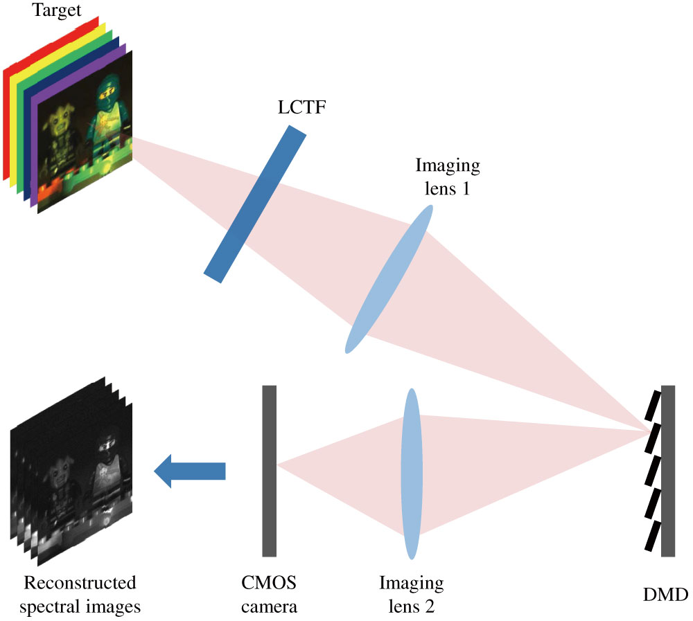
Fig. 1. Sketch of the LCTF-based hyperspectral imager.

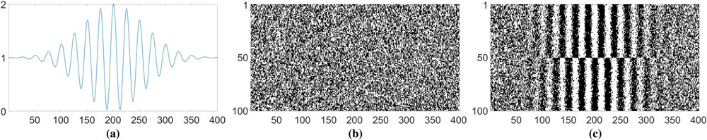
Fig. 2. Examples of different projection matrices (N=401,L=100) for the original signal shown in (a): (b) the random projection matrix and (c) the TACS projection matrix.

Fig. 3. Sequential scan of the spectral channels and compressive measurements using multiple coded snapshots. Note the coarse resolution of the detector array compared with that of the coded aperture.

Fig. 4. Method to generate the TACS coded apertures for the hyperspectral imaging systems.

Fig. 5. (a) Original reference image; (b) the recovered image using a random coded aperture; and (c), (d) a pair of the TACS coded aperture patterns generated based on (b).

Fig. 6. (a) Original spectral images, (b) the simulated low-resolution images obtained by conventional system, (c) the reconstructed spectral images using TACS coded apertures, and (d) the reconstructed spectral images using random coded apertures. Magnified details are presented as well.

Fig. 7. (a) RGB image of the scene, and (b)–(d) the original and reconstructed spectral signatures for three representative points, indicated by P1, P2, and P3 in (a).

Fig. 8. Influence of three key factors on the reconstruction performance. (a) The average reconstructed PSNRs in all spectral channels using different sub-group numbers, (b) the curves of average reconstructed PSNRs with respect to different compression ratios, and (c) the average PSNRs and (d) runtime corresponding to different reconstruction algorithms.

Fig. 9. Examples of coded patterns generated by (a) Galvis’s method and (b) Yang’s method.

Fig. 10. (a) Original spectral images in four spectral channels, (b) the reconstructed spectral images using the TACS coding method, (c) the reconstructed spectral images using Galvis’s method, and (d) the reconstructed spectral images using Yang’s method.

Fig. 11. Testbed of the staring hyperspectral imager with the proposed TACS coded apertures.

Fig. 12. (a) RGB image of the target used in the experiment; (b) an example of random coded aperture patterns; and (c), (d) the examples of TACS coded aperture patterns.

Fig. 13. (a) Original images in four spectral channels, (b) the low-resolution images obtained by the conventional system, (c) the reconstructed images obtained by TACS coded apertures, and (d) the reconstructed images obtained by random coded apertures. The color maps of the error patterns corresponding to (e) TACS coded apertures and (f) random coded apertures.

Fig. 14. Original and reconstructed spectra for two representative points indicated by P1 and P2 as shown in Fig. 12(a).

Fig. 15. (a) Original spectral images with center wavelengths of 554 nm, 563 nm, and 572 nm; (b) the simulated low-resolution images obtained by the conventional system; (c) the reconstructed spectral images using the proposed multi-channel method, and the reconstructed spectral images using the single-channel method with (d) TACS coded apertures and (e) random coded apertures.

Table 1. Comparison of Mean Values of μϒ and μϒ¯ Obtained by Random Projection Matrices and TACS Projection Matrices