Hyperspectral imaging acquires the spatio-spectral data cube of a scene over dozens to hundreds of narrow spectral bands [1,2]. Benefiting from the abundant spectral information, hyperspectral imaging has been used in a diverse range of applications from precision agriculture [3], food safety [4], medical diagnosis [5], to mineral mapping [6], and so on. Based on the data cube acquisition modes, hyperspectral imaging approaches can be classified into four categories known as whiskbroom [7], pushbroom [8], snapshot [9], and staring [10] approaches. Specifically, whiskbroom and pushbroom approaches are based on scanning in pointwise and linewise fashions, respectively. Snapshot approaches are proposed to multiplex the three-dimensional (3D) data cube onto a two-dimensional (2D) sensor, which is able to preserve the 2D spatial information as images typically have underlying spatial properties. However, there is a trade-off between the scanning process and spatial resolution [11]. To address this issue, staring hyperspectral imagers are well defined to capture the 2D spatial information of the scene at once, and sequentially scan the spectra using a rotating filter wheel or a tunable filter [12]. As they flexibly select the interested spectral range, staring approaches have been widely used in the field of hyperspectral imaging [13].

Recently, liquid crystal tunable filters (LCTFs) have been used as spectral bandpass filters in staring hyperspectral imagers attributed to their advantages of simple design, versatility, low wavefront distortion, flexible throughput control, faster speed, and large aperture with wide field of view [14–17]. However, the conventional LCTF-based hyperspectral imager is limited by the constant spatial resolution of its detector. In addition, high-resolution detectors may not be available in some cases [18]. Moreover, the substantial volume of hyperspectral images causes a dilemma for subsequent transmission and storage of the overall data [19]. The fast-emerging compressive sensing (CS) theory is well defined as a useful tool to reconstruct high-dimensional signals from much fewer multiplexed measurements than those required by the Nyquist sampling theorem, based on the sparse representation assumption [20–22]. Therefore, high-resolution images can be recovered from measurements on the low-resolution detector using the CS method [23]. In addition, compressive data are obtained during the acquisition stage, requiring less volume of total measurements than the original data cube. This benefits data transmission and storage. With these motivations, Wang et al. applied CS to develop a super-resolution LCTF-based hyperspectral imaging approach [24]. In Ref. [24], the spectral images were modulated in the spatial domain by a high-resolution random coded aperture, and then projected onto a low-resolution detector. However, random coding is suboptimal due to the sparse sensing matrix of the system, and thus the reconstruction performance can be improved with proper code design. Remarkably, the coded aperture determines the structure of the projection matrix in compressive sampling; thus it plays an important role in improving the reconstruction accuracy of the hyperspectral data cube [25,26]. The design of coded apertures has therefore attracted wide attention from researchers, remaining an important open issue in this field [27,28].

In the past, a set of numerical approaches has been developed to optimize the coded apertures based on the restricted isometry property [29,30] or empirical design rules [31,32]. However, the coded apertures in these methods are pre-designed before the data acquisition and cannot self-adapt to the characteristics of the underlying signal. In addition, the optimization methods entail high computational loads to the design process of spectral imaging systems. Recently, side information has been used to exploit non-local similarity [33], structural sparsity [34], rank minimization [35], etc. [36–39] to aid the reconstruction of undersampled signals. Learning from this concept, other approaches have been proposed to design the coded apertures based on a priori information of the underlying spectral images [40,41]. Nevertheless, these approaches require additional optical paths or auxiliary sensors to detect the side information of the spectral scene, which inevitably increase the complexity of the systems. In Ref. [42], Yang et al. proposed an adaptive CS sampling strategy based on the dictionary learned from the training data. However, the designed projection matrix in this method is not binary, which makes it difficult to implement in hardware.

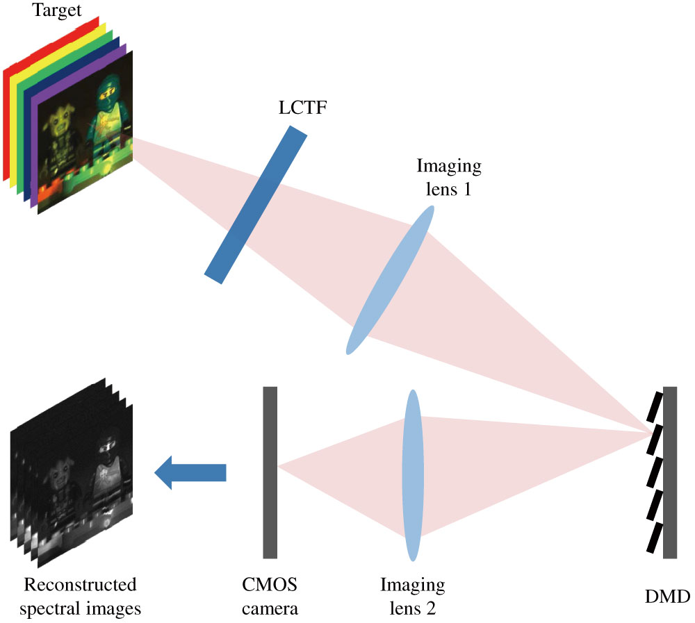
This paper proposes a two-tone adaptive CS (TACS) framework that can be easily implemented by coded apertures to enhance the spatial resolution and image quality of compressive spectral imaging systems. The sketch of the proposed hyperspectral imager is illustrated in Fig. 1. The light rays emitted from the target are incident upon the LCTF, which is used to successively select different spectral channels. The LCTF is considered an ideal spectral filter with narrow bandwidth that outputs a monochromatic image corresponding to its center wavelength [43]. The output of the LCTF is collected by the imaging lens 1, and then spatially modulated by a high-resolution coded aperture that is generated according to the TACS method. In hardware, the coded aperture patterns are implemented by the digital micromirror device (DMD). The DMD consists of an array of micromirrors that are individually controllable to generate different binary coded patterns [44–46]. Finally, the imaging lens 2 focuses the reflected light rays onto a low-resolution complementary metal oxide semiconductor (CMOS) detector. The CMOS detector is used to collect the compressive measurements, from which a high-resolution spectral image selected by the LCTF can be reconstructed. In order to obtain the 3D spectral data cube, the center wavelength of the LCTF needs to be tuned gradually to scan different spectral slices. Note that the proposed imager encodes the spectral images in the spatial domain, and thus spatial super-resolution is achieved while the number of acquired spectral channels remains the same. Because most of the hyperspectral images exhibit strong correlation among spectral channels, the spectra are assumed to be smooth [26,47]. Therefore, the recovered images from the previous spectral channels can be used as the reference images to construct the adaptive coded apertures for the following spectral channels. Given an a priori spectral image, a pair of complementary coded aperture patterns is generated by a reverse thresholding operation to respectively extract the structural characteristics of bright and dark regions. Since no extra side information of the spectral scene is needed, the proposed method does not increase the complexity of the imaging system. In addition, the computational complexity to calculate the adaptive coded apertures is negligible, compared to that of the conventional coded aperture optimization methods and the reconstruction process of the spectral images.

In order to further improve the reconstruction performance, multiple snapshots are carried out to increase the number of measurements. In the data acquisition process, the center wavelength of the LCTF is first fixed, and then different coded aperture patterns are switched successively on the DMD. In this paper, different coded aperture patterns are generated from one reference image using the random dithering method [48]. It is worth highlighting that the proposed TACS framework is proved theoretically to be valid based on the mutual-coherence criterion. In a statistical sense, the projection matrix for TACS is demonstrated to improve the sensing efficiency of the underlying signal. Simulation and experimental results verify the superiority of the proposed TACS coding method in terms of the imaging performance over the random coding method. In addition, comparison with other adaptive coding methods is provided to further assess the TACS coding method.

It should be noted that for the TACS method, each measurement encompasses the information of one spectral channel; thus only spatial compression is conducted. In order to compress the hyperspectral data cube in both spatial and spectral domains, the underlying concepts are extended to a multi-channel TACS method. During one integration time interval of the detector, the LCTF is switched for several times to encompass a series of spectral channels into one snapshot. In each snapshot, different spectral channels are modulated by different coded aperture patterns, then multiplexed and integrated on the CMOS detector. By doing so, each measurement includes the information of multiple spectral channels, thus increasing the compression capacity of the system. A set of simulations is conducted to prove the feasibility of the proposed multi-channel TACS method.

The remainder of this paper is organized as follows. Section 2 introduces the TACS framework. The proposed two-tone adaptive compressive hyperspectral imaging system is described in Section 3. Simulation and experimental results of the TACS method are provided in Section 4 and Section 5, respectively. The multi-channel TACS method is proposed and assessed in Section 6. Section 7 concludes the paper with some remarks.

It is known that most natural signals or images are sparse in some representation basis. Suppose X→∈RN×1 is a K-sparse signal in the basis Ψ=[ψ→1,ψ→2,…,ψ→N]∈RN×N; thus, it can be expressed as X→=ΨΘ→, where Ψ is the sparse basis, and Θ→∈RN×1 is the sparse coefficient vector including only K (K≪N) significant elements. Commonly used sparse bases include Fourier transform basis, discrete cosine basis (DCT), wavelet basis, and so on [49]. Let Y→ represent the compressive measurements of X→ given by Y→=ΦX→=ΦΨΘ→, where Φ=[ϕ→1,ϕ→2,…,ϕ→L]T∈RL×N is the projection matrix with L≪N. According to CS theory, the sparse signal X→ can be reconstructed from a few compressive measurements by solving the following inverse problem [20]: Θ→^=argminΘ→‖Θ→‖1,s.t.Y→=ΦX→=ΦΨΘ→,(1)where ‖·‖1 is the l1-norm, and Θ→^ is the reconstructed coefficient vector. Over the past years, a large number of algorithms have been proposed to effectively solve the optimization problem in Eq. (1) [50–52].

It then becomes natural to ask what properties the projection matrix Φ needs to satisfy to recover the signal successfully and accurately. Consider first the most general case where no a priori information of X→ is known. It has been shown that if Ψ is incoherent to Φ, X→ can be successfully recovered when the number of measurements satisfies L=C·K·logN≪N, where C≥1 is an oversampling factor [53]. The mutual coherence between Ψ and Φ can be evaluated by μ=max{|⟨ϕ→i,ψ→j⟩|2},i=1,2,…,Landj=1,2,…,N,(2)where ϕ→i is the ith row of Φ, ψ→j is the jth column of Ψ, and the vectors ϕ→i and ψ→j are normalized to have unit energy. It is remarkable that random projection matrices satisfy the incoherent property with high probability for almost all sparse signals [54].

However, in some other scenarios, some a priori information of X→ is known beforehand. For instance, an approximate (not exact) observation of the original signal is available, which can be exploited to improve the coding and reconstruction performance. To this end, Ma et al. introduced a design rule for the projection matrices based on the approximate observation of original signals [55]. First, the columns of the basis Ψ are separated into two sets: ϒ={ψ→l(1),ψ→l(2),…,ψ→l(K)} and ϒ¯, where l(i) indicates the location of the column corresponding to the ith non-zero coefficient, and ϒ¯ is the complementary set of ϒ. Accordingly, the mutual-coherence metric is divided into two parts: μϒ=maxψ→j∈ϒ{|⟨ϕ→i,ψ→j⟩|2} and μϒ¯=maxψ→j∈ϒ¯{|⟨ϕ→i,ψ→j⟩|2}. Given some a priori information of X→, it shows that a good projection matrix should maximize the difference between μϒ and μϒ¯ [55].

Monotone adaptive projection matrices were proposed in computational lithography to satisfy the aforementioned design rule, i.e., to maximize the difference between μϒ and μϒ¯ [55]. Suppose the observation of the original signal is given by S→=X→+ε→,(3)where ε→∈RN×1 is the noise vector. The elements of ε→ are independent identical random variables obeying the Gaussian distribution N(0,σX2) with zero-mean and variance σX2. The monotone adaptive projection matrix with ±1 elements can be constructed by thresholding the observation S→. However, the negative elements in the projection matrix cannot be physically implemented by the coded aperture used in the imaging system. That is because transmissive or reflective coded apertures modulate the amplitude of the incident wavefront without changing the phase.

To overcome this limitation, this paper proposes a TACS projection matrix with non-negative elements. The rows of the projection matrix Φ are independently generated by applying two-tone thresholding operations on the observation S→. Supposing the measurement number L is an even number, then the element of Φ in the ith row and jth column is defined as ϕ→ij={1+sgn(S→j−Λij)2Nif1≤i≤L21−sgn(S→j−Λij)2NifL2<i≤L,(4)where sgn(·) is the sign operator, S→j is the jth element of S→, and the threshold level Λij obeys the Gaussian distribution N(μΛ,σΛ2), where μΛ and σΛ2 are equal to the mean value and variance of S→, respectively.

The projection matrix defined in Eq. (4) constitutes two sub-projection matrices with all elements equal to 0 or 1. Figure 2 provides an intuitive illustration of different projection matrices (N=401,L=100) for the one-dimensional signal in Fig. 2(a). Figure 2(b) shows the conventional random projection matrix with Bernoulli sampling. Figure 2(c) illustrates the TACS projection matrix. In Figs. 2(b) and 2(c), the white and black pixels have the values of 1 and 0, respectively. Note that the TACS projection matrix extracts some structural characteristics of the original signal in Fig. 2(a), while the random projection matrix does not. In particular, the TACS projection matrix includes two sub-matrices. The top-half and bottom-half sub-matrices respectively capture the structural characteristics of the signal components beyond and below the threshold values. Thus, the overall compressive measurements capture the features of the entire signal.

Next, we use the design rule described in Subsection 2.A to assess the merit of the TACS projection matrix. Note that the voxels in hyperspectral images represent light intensities and thus they are always non-negative. This property will be used in the proof. In Appendix A, the proposed TACS projection matrix is proved to make the mean values of μϒ and μϒ¯ satisfy the following properties: $$\begin{gathered} μ¯ϒ=Δmaxψ→j∈ϒE{|⟨ϕ→i,ψ→j⟩|2}>‖X→‖222NK2θmax2, \\ μ¯ϒ¯=Δmaxψ→j∈ϒ¯E{|⟨ϕ→i,ψ→j⟩|2} \\ ≈14N{[2μXπ(σΛ2+σX2)∓1]∑m=1Nψ→^m}2, \end{gathered}$$(5)where E{·} represents the mathematical expectation; θmax represents the maximum element in the coefficient vector Θ→; and μX, σX2 correspond to the mean value and variance of X→, respectively. ψ→^m is the mth element in the vector ψ→^∈ϒ¯ that maximizes the mathematical expectation. In Appendix B, we further prove that if Ψ is chosen as the 2D-inverse DCT (IDCT) basis, then Eq. (5) becomes $$\begin{gathered} μ¯ϒ=maxψ→j∈ϒE{|⟨ϕ→i,ψ→j⟩|2}>‖X→‖222NK2θmax2, \\ μ¯ϒ¯=maxψ→j∈ϒ¯E{|⟨ϕ→i,ψ→j⟩|2}≈0. \end{gathered}$$(6)Equation (6) indicates that the proposed TACS projection matrix can separate μϒ and μϒ¯ in the statistical sense, thus making it satisfy the design rule.

Next, the superiority of the TACS projection matrix is verified by numerical simulations. Two signals with different dimensions are used as the original signals to be measured. Table 1 compares the mean values of μϒ and μϒ¯ obtained by the random projection matrices and TACS projection matrices. For each projection method, we repeat the simulations 100 times. In contrast to the random projection matrices, the TACS projection matrices further increase the difference between μϒ and μϒ¯, and satisfy the design rule better. Thus, the TACS projection matrix is apt to retain more information of the original signal than the random projection matrix, and benefits in improving the reconstruction performance.

As shown in Fig. 1, the LCTF-based hyperspectral imager consists of an LCTF, a DMD, and a CMOS detector. The input spatio-spectral data cube, f1(x,y,λ), is scanned in the spectral domain by tuning the center wavelength of the LCTF. This paper assumes that the LCTF is an ideal spectral filter, the output of which is considered a monochromatic image corresponding to the center wavelength of the LCTF. Suppose the transmission function of the LCTF is denoted as Tsnλ(λ). The output monochromatic image is expressed as f1nλ(x,y)=f0(x,y,λ)·Tsnλ(λ), where the superscript nλ(nλ=1,2,…,Nλ) represents the order number of the spectral channel. Then, the spectral images passing through the LCTF are spatially modulated by the binary coded aperture patterns, which are realized by the DMD. The DMD consists of an array of micromirrors. The tilt angle of each micromirror can be independently adjusted to change the direction of the reflected light rays. The block/unblock coded aperture patterns can be generated by flipping the corresponding micromirrors, and only the light rays reflected from the unblock pixels are collected to the main light path. The compressive measurement obtained on the detector plane can be written as $$\begin{gathered} gnλ(x,y)=∬f1nλ(x′,y′)·Tc(x′,y′)dx′dy′ \\ =∬f0(x′,y′,λ)·Tsnλ(λ)·Tc(x′,y′)dx′dy′, \end{gathered}$$(7)where Tc(x,y) represents the transmittance of the coded aperture.

In order to further improve the hyperspectral imaging performance, multiple snapshots are taken to increase the number of measurements. As shown in Fig. 3, the center wavelength of the LCTF is first fixed to select a certain spectral channel. In each spectral channel, the coded aperture pattern is switched for L times to capture L different compressive measurements. Afterwards, we tune the center wavelength of the LCTF to the next spectral channel and repeat the measurement process mentioned above. After scanning all the spectral channels, the measurement procedure is terminated. In this case, the coded aperture pattern is denoted as Tcl(x,y), where l=1,2,…,L indexes the order number of snapshots. Thus, the lth compressive measurement in the nλth spectral channel, referred to as gnλ,l(x,y), is formulated as gnλ,l(x,y)=∬f0(x′,y′,λ)·Tsnλ(λ)·Tcl(x′,y′)·dx′dy′.(8)

To simplify the analysis of the system, the imaging model in Eq. (8) is reformulated into a discrete form. The hyperspectral data cube is gridded into Nx×Ny×Nλ voxels. Each voxel is denoted as Fnx,ny,nλ, where nx,ny represent the spatial coordinates (nx=1,2,…,Nx and ny=1,2,…,Ny). The requirement for super-resolution is that the pitch resolution of the DMD should be higher than that of the CMOS detector. Specifically, let Δc and Δd be the pitch sizes on the coded aperture and the detector, respectively. Then, the ratio of resolution between the coded aperture and the detector is defined as R=Δd/Δc. Assume R is a positive integer larger than 1. That is, the dimension of the coded aperture is Nx×Ny, and the dimension of the detector is Mx×My, where Nx/Mx=Ny/My=R. Thus, the overall compression ratio is defined as γo=γc·L=(1/R)2·L, where γc refers to the compression ratio for one snapshot. In the lth snapshot, the measurement on the (mx,my)th pixel of the detector is represented by Gmx,mynλ,l. The discrete version of the imaging model in Eq. (8) can be written as Gmx,mynλ,l=∑nx=R(mx−1)+1Rmx∑ny=R(my−1)+1RmyFnx,ny,nλ·Tnx,ny,nλnλ,l,(9)where mx=1,2,…,Mx, my=1,2,…,My, and Tnx,ny,nλnλ,l denotes the discrete transmittance of the LCTF and coded aperture corresponding to the voxel (nx,ny,nλ).

Alternatively, the hyperspectral data cube can be expressed as its vector representation across Nλ spectral channels. Let f→nλ∈RNx·Ny×1 denote monochromatic image in the nλth spectral channel, which is sparse in a basis Ψ∈R(Nx·Ny)×(Nx·Ny), such that f→nλ=ΨΘ→nλ. Assume g→nλ∈RL·Mx·My×1 is the vectorized representation of the measurement G in the nλth spectral channel. Following this notation, the imaging model in Eq. (9) can be rewritten as g→nλ=Φnλf→nλ+ρ→nλ=ΦnλΨΘ→nλ+ρ→nλ,(10)where ρ→nλ∈RL·Mx·My×1 represents the measurement noise. Φnλ∈R(L·Mx·My)×(Nx·Ny) is the spatial transmission matrix of the coded aperture for the nλth spectral channel, and it is constructed from the following: Φnλ=[Φnλ10…00Φnλ2…0⋮⋮⋱⋮00…ΦnλMx·My],(11)where Φnλi∈RL×R2(i=1,2,…,Mx·My) denotes the transmission matrix corresponding to the ith detector pixel, and 0∈RL×R2 represents the zero matrix.

Thus, the coefficient vector of the hyperspectral image in the nλth spectral channel can be reconstructed from the following inverse optimization problem: Θ→^nλ=argminΘ→nλ‖Θ→nλ‖1,s.t.‖g→nλ−ΦnλΨΘ→nλ‖2≤β,(12)where ‖·‖2 is the l2-norm, and β is the bound of noise. Due to the advantage in reconstruction quality, the gradient projection for sparse reconstruction (GPSR) algorithm is used to solve the optimization problem [50]. Other reconstruction algorithms proposed in the CS realm, such as the two-step iterative shrinkage/thresholding (TwIST) algorithm [51] and the sparse reconstruction by separable approximation (SpaRSA) algorithm [52], can also be used.

Next, we describe how to generate the TACS coded apertures during the measurement process. Because the hyperspectral images exhibit strong correlation among spectral channels, that is, the spectra are smooth, the images in the adjacent spectral channels should have similar structural characteristics [56]. Therefore, we can divide the entire spectra into several sub-groups, each of which includes several adjacent spectral channels. As shown in Fig. 4, for each sub-group, one reference spectral channel is selected and reconstructed using a random coded aperture. After that, the reconstructed reference image is used as the a priori information to construct the TACS coded aperture for all spectral channels in this sub-group.

To explain this process more clearly, let us take a special case, i.e., Mx·My=1. The images within the Nuth and Nvth spectral channels belonging to the same sub-group are denoted by INu∈RNx×Ny and INv∈RNx×Ny, respectively. Assume the Nuth spectral channel is the reference channel. Then, the reconstruction of INu denoted by I^Nu is used as the a priori information to design the TACS coded aperture for the spectral image INv. Define an operator vec(·) that transforms an image into its vectorized representation by stacking all the columns. Due to the similarity between the adjacent spectral images, we have vec(I^Nu)≈vec(INv)+ε→, where ε→ denotes the error term. Compared to Eq. (3), vec(INv) and vec(I^Nu) can be regarded as the original signal X→ and its approximate observation S→, respectively. Let N=Nx·Ny, and we can generate L different adaptive projection vectors with length of N according to Eq. (4). After that, these projection vectors are inversely stacked into L different 2D TACS coded aperture patterns with dimension of Nx×Ny. In practice, we can reconstruct every R×R sub-region on the spectral images independently, and then stitch them up to obtain the full spectral images. In this case, Φnλi in Eq. (11) is generated in accordance with the same process as mentioned above. Each row of Φnλi is denoted by ϕnλi,l∈R1×R2, which represents the transmission function for the ith spatial pixel on the detector in the lth snapshot. That is, Φnλi=[(ϕnλi,1)T,(ϕnλi,2)T,…(ϕnλi,L)T]T. Then, ϕnλi,l can be stacked into an R×R matrix denoted by Πnλi,l. Note that Πnλi,l represents the R×R sub-region on the coded aperture for the lth snapshot. Stitching up the sub-matrices Πnλ1,l,Πnλ2,l,…,ΠnλMx·My,l together, we can obtain the lth coded aperture pattern.

In this subsection, two sets of simulations are conducted using the real hyperspectral data, where the reconstruction performance obtained by TACS coded apertures and random coded apertures is compared. In the following simulations, the Lego figures are used as the target, and the original hyperspectral data cube consists of 256×256 pixels in the spatial domain and 24 spectral bands. More specifically, the center wavelengths of the 24 spectral bands are 450 nm, 459 nm, 467 nm, 476 nm, 485 nm, 493 nm, 502 nm, 511 nm, 520 nm, 528 nm, 537 nm, 546 nm, 554 nm, 563 nm, 572 nm, 580 nm, 589 nm, 598 nm, 607 nm, 615 nm, 624 nm, 633 nm, 641 nm, and 650 nm, respectively. The intensity of the test data is normalized to the range of [0,1]. The coded aperture includes 256×256 pixels, while the detector constitutes 32×32 pixels. Thus, every 8×8 pixels on the coded aperture correspond to one detector pixel and γc=(1/8)2. The measurement error on the detector is emulated by the white Gaussian noise with signal-to-noise ratio (SNR) level of 30 dB. In the reconstruction process, the 2D-IDCT basis is used to sparsely represent the spectral images. All of the calculations are carried out using MATLAB R2016a on a server with Intel Xeon E3-1505M v5 2.8 GHz processor, and 64 GB memory.

According to Section 3, we first divide the entire spectra evenly into four sub-groups and reconstruct one reference spectral channel in each sub-group. At this point, the number of snapshots L is set to 32. Figures 5(a) and 5(b) show an original reference image and its reconstruction result using a random coded aperture. Taking the recovered reference image as the a priori information, the TACS coded aperture patterns are generated for all spectral channels in the same sub-group. A pair of the TACS coded aperture patterns is shown in Figs. 5(c) and 5(d). It can be easily observed that these two coded aperture patterns are approximately complementary, and respectively extract the structural information within bright and dark regions. Next, the TACS coded apertures are used to modulate and reconstruct the spectral images with multiple snapshots (L=12). Thus, the overall compression ratio is γo=0.1875.

Figure 6 presents the spectral images obtained by the conventional system and the reconstructed spectral images obtained by different kinds of coded apertures for comparison. Figure 6(a) illustrates the high-resolution original images of four spectral channels in the data cube. Figure 6(b) shows the low-resolution images captured by the conventional system, which cannot achieve super-resolution without using the theory of CS. The low-resolution images are simulated by downsampling the original images along both horizontal and vertical directions with a scaling factor of 8, and their spatial resolution is 32×32 pixels. And they are presented to demonstrate the resolution improvement brought by the compressive imaging system. Figures 6(c) and 6(d) show the reconstructed spectral images consisting of 256×256 pixels using TACS coded apertures and random coded apertures, respectively. Note that in Fig. 6(d), the spectral images are reconstructed with 12 snapshots to make a fair comparison. The peak SNRs (PSNRs) of the reconstructed images are also presented in the figure. The proposed TACS coded apertures are shown to effectively improve the reconstruction quality compared to the random coded apertures under the same compression ratio. In order to clearly illustrate the improvement, the specific regions around the eyes are magnified in Fig. 6. Figure 7 plots the original and reconstructed spectral signatures for three representative points on the target. The three representative points are selected from different colorful regions, as shown in Fig. 7(a). The intensities in Figs. 7(b)–7(d) indicate the normalized values of the spectra at those three spatial points. The TACS coded apertures are proved to achieve superior fidelity of the spectral reconstructions over the random coded apertures. It shows that these reconstructed spectral signatures are smooth, which implies that the proposed method is reasonable to use the reconstructed images from previous spectral channels as a priori information.

The impact of some key factors on the reconstruction performance is studied in this subsection. Three key factors considered are the number of sub-groups, the compression ratio, and the reconstruction algorithm. Figure 8(a) illustrates the average reconstructed PSNRs in all spectral channels using the TACS method with different sub-group numbers. In addition, the PSNR curve obtained by random coded apertures is also provided for comparison. For each curve, the reconstruction simulations are repeated three times, and the average PSNRs of the reconstructed images are calculated. In general, the quality of the reconstructed images is enhanced when more sub-groups are used. Increasing the number of sub-groups will decrease the number of adjacent spectral channels in each sub-group. Thus, the similarity among the spectral images within each sub-group will also be improved. Since all spectral images in a sub-group are modulated and reconstructed based on one reference image, increasing the number of sub-groups will improve the reconstruction accuracy. However, dividing the entire spectra into more sub-groups will also increase the computational complexity. That is because one reference spectral channel is required to be reconstructed using a random coded aperture for each sub-group. Given the number of sub-groups Sg, we need to reconstruct Sg reference spectral channels. Moreover, different sub-groups use different sets of adaptive coded apertures. Then Sg adaptive coded apertures need to be generated. Thus, the computational complexity to generate the adaptive coded apertures is proportional to the number of sub-groups.

Afterwards, we repeat the simulations in Fig. 6 using different compression ratios. The curves of average reconstructed PSNRs over the four spectral channels with respect to different compression ratios are shown in Fig. 8(b). As can be noticed, the TACS coded apertures outperform the random coded apertures in the reconstruction performance under different compression ratios. In addition, the advantage of TACS coded apertures becomes more obvious as the compression ratio reduces. That is because the TACS coded apertures can extract the structural characteristics of the target and retain more information of the spectral data cube in the compressive measurements. For instance, when the compression ratio reduces to 0.1, the TACS coded apertures obtain 5.16 dB gain on the average PSNR over the random coded apertures.

Furthermore, simulations are conducted using the TACS coded apertures to compare the reconstruction quality and computational efficiency of different reconstruction algorithms. The settings of the simulation are the same as those in Fig. 6. For each algorithm, we repeat the reconstructions three times, and calculate the average PSNRs and runtime. Figures 8(c) and 8(d) present the average PSNRs and runtime corresponding to the GPSR algorithm, TwIST algorithm, and SpaRSA algorithm, respectively. It is observed that the GPSR algorithm can achieve the best reconstruction performance. Although the computational efficiency of the GPSR algorithm is lower than that of TwIST and SpaRSA algorithms, it is still fast to handle the reconstruction problem. The TwIST algorithm leads to the shortest runtime, but the reconstruction performance is much worse than that of the other two algorithms, especially in the spectral channels with shorter wavelengths.

This subsection provides the simulation results of two other adaptive coding methods to further illustrate the superiority of the TACS coded apertures. In Ref. [40], Galvis et al. estimated the edge of the scene using the image obtained from a red–green–blue (RGB) sensor and subsequently designed the structured coded aperture. They applied two different blue-noise coded patterns to the edge and non-edge regions in order to improve the reconstruction quality of the feature boundaries. Yang et al. proposed an adaptive sampling strategy for hyperspectral images based on dictionary learning in Ref. [42]. Specifically, they first learned the over-complete dictionary from the training data, and then computed a singular value decomposition from the dictionary. And a small number of left singular vectors were used eventually as the rows of the projection matrix.

Based on the foundation of their work, we simulate these two methods using our proposed framework. Adaptive coded patterns are generated by replacing the RGB images in Galvis’s method and the training data in Yang’s method with the recovered images from previous spectral channels. Figures 9(a) and 9(b) respectively present examples of the coded patterns generated by Galvis’s method and Yang’s method.

Next, the data cubes are recovered from a small set of measurements, according to the same process and settings as Subsection 4.A. Figure 10(a) illustrates the original images of four spectral channels in the data cube. The reconstructed spectral images using the TACS coding method, Galvis’s method, and Yang’s method are respectively shown in Figs. 10(b)–10(d). The average PSNRs for the entire reconstructed data cubes using Galvis’s and Yang’s methods are 27.64 dB and 30.39 dB, respectively. As can be noticed, the reconstruction performance using Galvis’s method is inferior to the TACS coding method. That is because the content information of the RGB image in the non-edge regions is not fully utilized. In addition, the proposed TACS coding method outperforms Yang’s method. But the gap is not so obvious since the dictionary is also adaptively learned from the a priori information in Yang’s method. However, the process of dictionary learning is time-consuming and the coded patterns in Yang’s method are not binary, thus making it inapplicable for hardware implementation.

This section demonstrates the proposed TACS coded apertures on an experimental testbed of a staring hyperspectral imager developed by our group. As shown in Fig. 11, the testbed consists of an RL127-WHI-IC broadband ring light source (Edmund), a VNIR-5/20-20-S LCTF (Wayho Technology), two AC254-050-A imaging lenses (Thorlabs) with a focal length of 50.2 mm, a DLP9500 DMD (Texas Instruments), and an acA2040-90μm monochromatic CMOS camera (Basler) to capture the measurements. The CMOS camera consists of 1024×1024 pixels with a pitch size of 11.0 μm. The DMD includes 1920×1080 micromirrors with a pitch size of 10.8 μm.

The system should be calibrated beforehand. During the calibration process, the distances between optical components were adjusted to obtain one-to-one correspondence between the coded aperture pixels and detector pixels. In addition, the effect of dark noise was eliminated, and the non-uniformity of the light source was corrected. Taking into account the effects of system impulse response and stray light, the coded aperture patterns were first measured and recorded when the target was replaced by a diffuse plate. Then, the normalized detected patterns were regarded as the actual transmission functions of the coded apertures. When all of the micromirrors on the DMD were turned on, the measurements of the CMOS detector without spatial coding were considered the original images of the target.

As described in Subsection 4.A, the entire spectra are evenly divided into four sub-groups. The real target under detection is shown in Fig. 12(a). In the measurement stage, a resized region including 400×400 pixels on the DMD was used to implement the coded apertures. Figure 12(b) illustrates an example of random coded aperture patterns used to reconstruct the reference spectral image, and Figs. 12(c) and 12(d) illustrate the examples of TACS coded aperture patterns generated according to the reference image. Compared with the random coded apertures, TACS coded apertures extract the structural characteristics of the scene effectively. To reconstruct the reference spectral channels, 32 snapshots were carried out using random coded apertures. Then, 12 snapshots were taken with the TACS coded aperture patterns to reconstruct all of the spectral images within the same sub-group. The center wavelength of the LCTF was tuned for 24 times in total to obtain 24 spectral bands, from 515 nm to 630 nm with an interval of 5 nm. In order to emulate the low-resolution detector, all 8×8 pixels on the detector were combined into one macro-pixel, and then 50×50 macro-pixels were used to acquire the measurement data.

As a comparison, we also built the testbed of the conventional spectral imaging system without using CS theory. In the conventional system, all the micromirrors on the DMD were set to unblock, so that the incident light was directly reflected to the main optical path. In order to acquire the data cube, the LCTF was switched for 24 times to obtain 24 spectral images, each of which consists of 50×50 pixels. For the conventional system, the time to collect the full data is 10 s, while it costs 166 s to acquire all compressive measurements of 24 spectral bands using 12 TACS coded aperture patterns. That is because multiple snapshots are taken to improve the reconstruction quality of super-resolution images for the TACS method.

Figure 13 illustrates the spectral images obtained by different methods using the experimental testbed. The original images in four spectral channels are presented in Fig. 13(a), and the spatial resolution of these images is 400×400 pixels. Figure 13(b) shows the images containing 50×50 pixels acquired by the conventional system. The conventional system does not utilize the CS theory; thus its spatial resolution is determined by the low-resolution detector. The reconstructed spectral images using TACS coded apertures and random coded apertures both with 12 snapshots are respectively shown in Figs. 13(c) and 13(d). The corresponding PSNRs of the reconstructed images are also presented in the figure. The average PSNRs for the entire reconstructed data cube using TACS and random coded apertures are 23.80 dB and 20.59 dB, respectively. To make the comparison more clear, the error patterns of the recovered images with respect to the original images are illustrated in Figs. 13(e) and 13(f). In more detail, Figs. 13(e) and 13(f) show the color maps of error patterns corresponding to the TACS coded apertures and random coded apertures, respectively. Every pixel in the error pattern represents the absolute intensity error of the corresponding pixel between the reconstructed image and the original image. In addition, the mean square errors of all error patterns are presented in Fig. 13. It is observed that the TACS coded apertures achieve superior reconstruction quality over the random coded apertures. Appendix C provides the comparison among these different methods using the experimental testbed in detail.

Figure 14 plots the original and reconstructed spectra of two representative points on the target located at P1 and P2 in Fig. 12(a). The spectra are characterized by the reflectances, which are obtained through spectral calibration and have no units. And the original spectral reflectances are measured by an HR4000 grating spectrometer (Ocean Optics). It is shown that the reconstructed spectra using the TACS coded apertures are more consistent with the original spectra. As illustrated in Fig. 14, the spectra are smooth, which confirms the correlation characteristic among the neighboring spectral channels again.

In the above sections, only one spectral channel is captured during one integration time interval of the detector. This section proposes a multi-channel TACS method to introduce the spectral compression and maintain the reconstruction quality without changing the structure of the imaging system. During one integration time interval of the detector, the LCTF is tuned for several times to encompass a series of spectral channels into one snapshot, each of which is modulated by different coded aperture patterns loaded on the DMD. Then, the coded images in these spectral channels are projected and integrated on the CMOS detector. In this way, spectral images in multiple channels, rather than just one channel, are involved in each measurement, thereby increasing the compression capacity of the system. Different from Section 3, the overall compression ratio is determined by γom=γo·1Q=LR2·Q,(13)where Q represents the number of times to switch the LCTF during each integration time interval, and Q<Nλ. Compared to the single-channel method described in Section 3, the compression capacity of the system is increased by Q-fold.

Suppose the spectral images within the N1th,N2th,…,NQth channels are collected during one integration time interval, and all of them belong to the same sub-group. Then, the imaging model based on the multi-channel method is reformulated as follows: g→m=Φmf→m+ρ→m=ΦmΨmΘ→m+ρ→m,(14)where g→m represents the measurements using the multi-channel method; f→m is the raster-scanned vector of the spectral images in those NQ channels, i.e., f→m=[(f→N1)T,(f→N2)T,…,(f→NQ)]T∈RQ·Nx·Ny×1; Ψm=diag(ΨN1,ΨN2,…,ΨNQ)∈R(Q·Nx·Ny)×(Q·Nx·Ny); ρ→m∈RL·Q·Mx·My×1 denotes the measurement noise; and Φm∈R(L·Mx·My)×(Q·Nx·Ny) can be expressed as Φm=[Φm10…00Φm2…0⋮⋮⋱⋮00…ΦmMx·My],(15)where 0 represents a zero matrix of order L×QR2. It is noted that Φmi∈RL×QR2(i=1,2,…,Mx·My) is constructed as Φmi=[ΦN1i,ΦN2i,…,ΦNQi],(16)where ΦNji(j=1,2,…,Q) refers to the transmission sub-matrix for the Njth spectral channel. As mentioned in Section 3, all spectral channels in the same sub-group share the same set of TACS coded aperture patterns. That means ΦNji remains unchanged within the same sub-group. However, in the multi-channel method, spectral images in different channels need to be modulated by different coded apertures. So for the Njth channel, the corresponding ΦNji is respectively generated according to Section 3. Thus, f→m can be reconstructed by solving the problem in Eq. (14). After that, we can obtain the spectral images in different channels by decomposing f→m into f→N1,f→N2,…,f→NQ.

Next, we provide the simulation results of the proposed multi-channel method. The reference spectral channels are obtained and reconstructed as described in Subsection 4.A. And all parameters are the same as those used in Subsection 4.A. In particular, we capture three spectral channels during each integration time interval, that is Q=3. Thus, the overall compression ratio is γom=0.0625, and the measurement number is reduced to one third of that used for the single-channel method. Figure 15(a) shows the original spectral images with center wavelengths of 554 nm, 563 nm, and 572 nm. The simulated low-resolution images obtained by the conventional system are shown in Fig. 15(b) to illustrate the improvement in spatial resolution. The reconstructed spectral images using the multi-channel method are presented in Fig. 15(c). Figures 15(d) and 15(e) illustrate the reconstructed spectral images using the single-channel method with TACS coded apertures and random coded apertures, respectively. The average PSNR for the entire reconstructed data cube using the multi-channel method is 28.98 dB. Compared to the single-channel method with random coded apertures, the proposed multi-channel method can improve the reconstruction quality. However, the reconstruction performance is inferior to the single-channel method with TACS coded apertures, since the reduction of measurements will degrade the image quality. It can be concluded that the proposed multi-channel method can improve the compression capacity of the system, while maintaining the reconstruction quality to a certain extent. In Appendix D, a side-by-side comparison of the three coding methods is summarized. In the future, experiments will be done to verify the multi-channel method.

This paper developed a novel TACS coding method in spectral imaging and demonstrated it based on the LCTF-based hyperspectral imager for the first time. CS theory was used to obtain the high-resolution hyperspectral data cube that can be recovered from a small set of measurements on the low-resolution detector. Meanwhile, the proposed TACS coded apertures can achieve superior reconstruction performance over the random coded apertures, since the TACS coded apertures can capture the structural characteristics of the underlying target. Moreover, it was proven that the TACS coding method satisfies the mutual-coherence metric better than the traditional random coding method. Using the proposed TACS coding, an improvement up to 4.81 dB on the average reconstructed PSNR is observed in the simulations. In addition, simulation results of other adaptive coding methods are provided for further comparison. Then experiments on the testbed were carried out and the superiority of the proposed TACS coded apertures was demonstrated. Finally, the multi-channel TACS method was proposed to compress the hyperspectral data cube in the spatial and spectral domains simultaneously. The developed super-resolution staring hyperspectral imager was shown to provide promising image quality using the cost-effective low-resolution detectors.