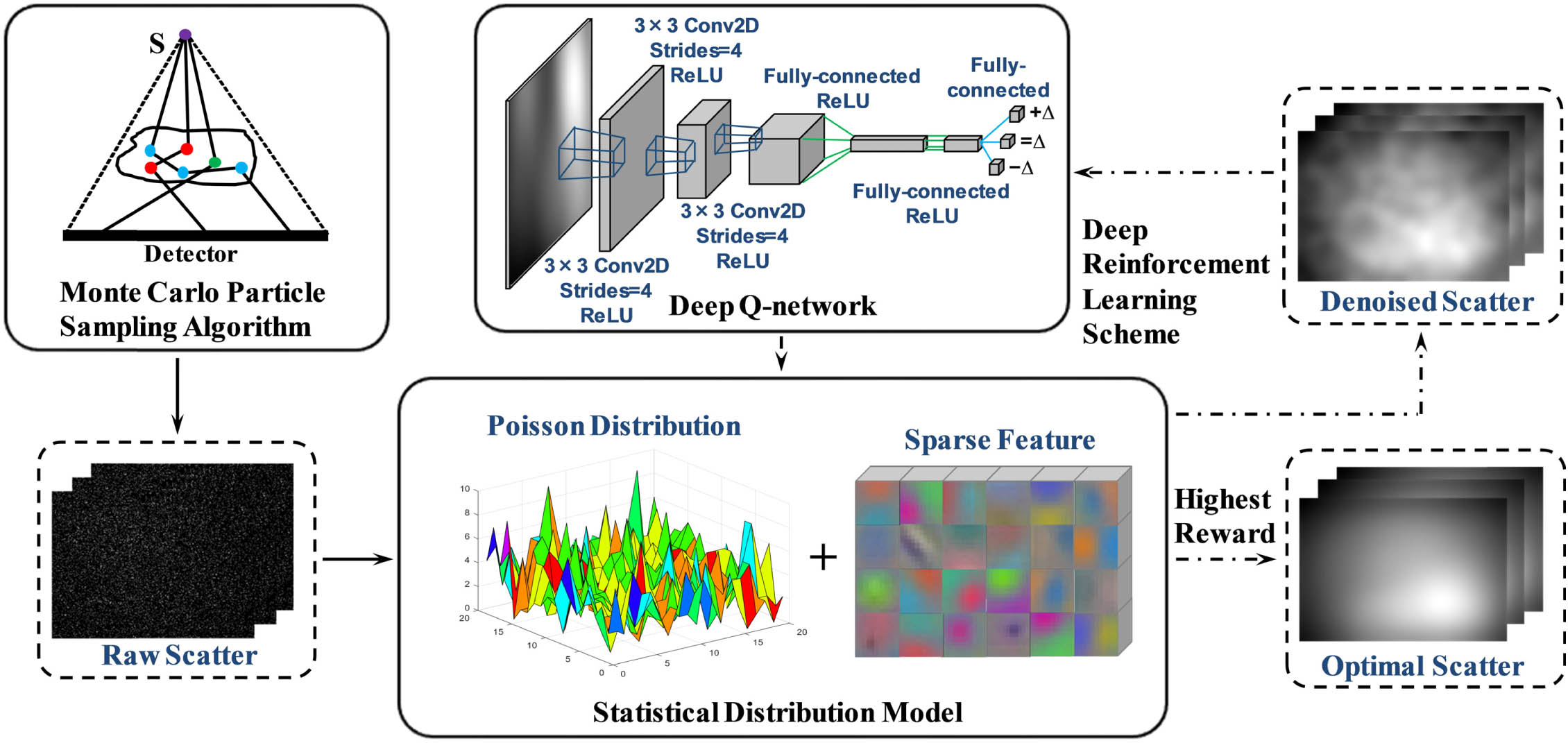
Fig. 1. Automatic scatter estimation framework. The MC algorithm generates raw scatter signals in terms of the X-ray source energy spectrum and system geometry configuration. The DRL scheme (denoted by the dashed black arrow) employs a deep Q-network to interact with the statistical distribution model to yield a satisfactory scatter image.

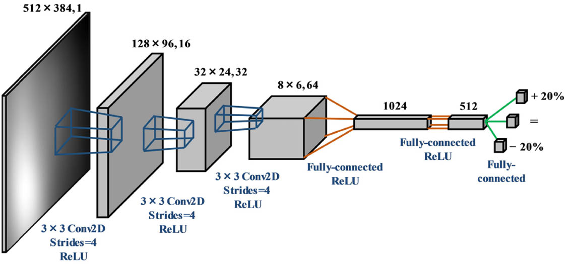
Fig. 2. Network architecture in the DDQN. The network takes a scatter image as input and predicts three possible actions for parameter adjustment. The number at the top denotes the feature map size and channel number, and the operations for each layer are presented at the bottom. For instance, the first hidden layer convolves 16 filters of 3×3 with stride four with the input layer followed by a rectified linear unit (ReLU) activation function, and the output layer is a fully connected linear layer with three outputs.

Fig. 3. (a) is the primary projection of the head and neck (H&N) patient; (b)–(i) represent raw scatter projections that are separately calculated by the MC particle sampling algorithm with source photons of 5×105, 1×106, 5×106, 1×107, 1×108, 1×109, 1×1010, and 1×1012 for the same projection angle.

Fig. 4. (a)–(g) are the scatter images of Figs. 3(b)–3(h) smoothed by the over-relaxation smoothing algorithm; (h) corresponds to Fig. 3(i), which is considered a noise free scatter image and utilized as the ground truth.

Fig. 5. Intensity profiles of Fig. 4 along the (a) horizontal and (b) vertical directions as denoted by the orange lines in Fig. 4(h).

Fig. 6. From top to bottom: six testing results with 5×105, 1×106, 5×106, 1×107, 1×108, and 1×109 source photons. From left to right: primary signals, smoothed scatter signals restored by the over-relaxation algorithm with empirical parameters, smoothed scatter signals restored by the proposed framework, and the ground truth.

Fig. 7. (a)–(d) Intensity profiles of the first, second, third, and last rows in Fig. 6. The locations of the profiles (a)–(d) are denoted by orange lines at the last column of Fig. 6.

Fig. 8. (a)–(c) indicate boxplots of the metric difference of SSIM, PSNR, and RAE between Empirical and ASEF for all testing cases. metricdiff=metricEmpirical−metricASEF, where metric denotes SSIM, PSNR, and RAE, respectively. (d) is the boxplot of the SSIM comparison of Empirical and ASEF.

Fig. 9. Automatic scatter estimation process for a testing case. (a)–(c) are smoothed scatter images at Steps 1, 7, and 13, respectively. (d) and (e) separately plot the SSIM and RAE over steps.

Fig. 10. Different scatter images. From left to right: scatter projection input, the ground truth of the scatter image at the first column, and Grad-CAM heatmaps of three subnetworks {Wk,Wω,Wβ}.

Fig. 11. From top to bottom: four prostate cases with 5×105, 1×106, 5×106, and 1×107 source photons. From left to right: primary signals, smoothed scatter signals restored by the over-relaxation algorithm with empirical parameters, smoothed scatter signals restored by the proposed framework, and the ground truth.

Fig. 12. (a)–(d) Intensity profiles of the four prostate cases presented in Fig. 11. Profile locations are outlined by orange lines in the last column of Fig. 11.

Table 1. DDQN Training Process

Table 2. Parameters in the DDQN Training Phase

Table 3. SSIM, PSNR, and RAE Statistics (avg.±std.) among All Testing Cases^a

Table 4. Computation Time for One Scatter Image of a Prostate Patient across Different Photon Numbers