Jianhui Ma, Zun Piao, Shuang Huang, Xiaoman Duan, Genggeng Qin, Linghong Zhou, Yuan Xu, "Monte Carlo simulation fused with target distribution modeling via deep reinforcement learning for automatic high-efficiency photon distribution estimation," Photonics Res. 9, B45 (2021)
Copy Citation Text
Particle distribution estimation is an important issue in medical diagnosis. In particular, photon scattering in some medical devices extremely degrades image quality and causes measurement inaccuracy. The Monte Carlo (MC) algorithm is regarded as the most accurate particle estimation approach but is still time-consuming, even with graphic processing unit (GPU) acceleration. The goal of this work is to develop an automatic scatter estimation framework for high-efficiency photon distribution estimation. Specifically, a GPU-based MC simulation initially yields a raw scatter signal with a low photon number to hasten scatter generation. In the proposed method, assume that the scatter signal follows Poisson distribution, where an optimization objective function fused with sparse feature penalty is modeled. Then, an over-relaxation algorithm is deduced mathematically to solve this objective function. For optimizing the parameters in the over-relaxation algorithm, the deep -network in the deep reinforcement learning scheme is built to intelligently interact with the over-relaxation algorithm to accurately and rapidly estimate a scatter signal with the large range of photon numbers. Experimental results demonstrated that our proposed framework can achieve superior performance with structural similarity , peak signal-to-noise ratio , and relative absolute error , and the lowest computation time for one scatter image generation can be within 2 s.
1. INTRODUCTION
Particle distribution estimation is an important issue in medical diagnosis because the principle of that distribution in some crucial imaging devices follows the law of large numbers [1]. However, particle distribution estimation by only trillions of particle sampling is extremely time-consuming. Thus, approximating a target function model on the basis of target distribution feature analysis can substantially hasten particle estimation [2]. Particles fused with a target distribution feature for a few particles have a promising prospect in rapid statistical estimation without the loss of accuracy. As an important branch of particle distribution estimation, photon scattering is commonly involved in X-ray imaging, especially cone beam computed tomography (CBCT), which has been widely used in medical imaging given its high spatial resolution and low radiation dose and for applications such as dental CBCT, image-guided radiotherapy, and extremity CBCT [3]. Scatter occurs when photons emitted from an X-ray source interact with a physical object and can extremely degrade the reconstructed image quality for clinical diagnosis, thereby leading to pixel-value inaccuracy. Various methods have been proposed for scatter removal, including the scatter kernel [4,5], beam stop array technique [6,7], and primary modulator [8]. Nevertheless, these approaches require additional equipment or increase the irradiation dose to the patient. The Monte Carlo (MC) particle sampling approach has been proved to estimate accurate scatter signals in a cost-efficient manner without the above disadvantages [9–11]. The said technique can precisely simulate the physical process of photon transport to produce all types of scatters composed of Compton, Rayleigh, and photoelectric effect. In reality, one X-ray tube generates approximately source photons for imaging one projection under one angle view. Therefore, the scatter simulation of photon transport by only MC particle sampling is extremely time-consuming, and this feature precludes its clinical application [12].
To enhance its computational efficiency, the scatter signal is typically simulated by an MC algorithm with a low photon number, so the generated signal is noisy and fragmentary. To overcome this problem, the noise-contaminated scatter signal is assumed to be governed by the Poisson distribution and sparse feature representation. An efficient denoising algorithm based on Poisson distribution and sparse feature fusion is proposed to smooth the signal along the spatial dimension. Nonetheless, the weight parameter between the Poisson distribution and sparse feature does not follow a one-size-fits-all trend for all cases with different photon numbers. Tuning parameters manually for all situations is a trial-and-error process, which calls for considerable time and effort. Moreover, that scheme hinders a noise removal algorithm from reaching an optimal solution of generating an accurate scatter signal via ultra-low photons.
In the past few years, deep-learning algorithms have achieved remarkable success across many fields, such as computer vision and pattern recognition [13–18]. Deep-learning methods build deep neural networks (DNN) to directly extract local and global features from the dataset, an approach that can avoid handcrafted selection [13]. Motivated by the powerful performance of deep learning, the Google DeepMind group integrated a neural network and reinforcement learning (RL) algorithm to play Atari games with human-level performance [19]. Afterwards, AlphaGo based on deep RL (DRL) defeated human masters in the ancient Chinese game and attracted global attention [20]. Shen et al. [21] proposed a parameter tuning policy network to adjust pixel-wise parameters in iterative computed tomography (CT) reconstruction and attain comparable or better image quality. DRL was also applied in radiotherapy for optimal dose adaptation and a treatment planning optimization problem [22–25]. These superior performances have demonstrated that the DRL algorithm can achieve a task analogous to human instincts. In DRL, an agent represented by a DNN interacts with the environment to explore all possible consequences of the action for the highest reward feedback. The agent acts according to their observation of the environment, which, in turn, is changed by the action and yields a new observation for the next step. Over many episodes, the agent is supposed to develop an optimal policy to obtain maximum rewards. Essentially, parameter tuning is a dynamic decision-making process, for which DRL is highly suitable. Inspired by the impressive achievements of pioneering work and the rationale of DRL, we propose a framework to realize automatic high-efficiency scatter estimation via the fusion of MC particle sampling, statistical distribution features, and a DRL scheme.
Sign up for Photonics Research TOC. Get the latest issue of Photonics Research delivered right to you!Sign up now
The remainder of this paper is organized as follows. Section 2 describes the automatic scatter estimation framework (ASEF), including its key components, namely, the MC particle sampling algorithm, Poisson distribution and sparse feature-based statistical distribution algorithm, and a DRL scheme. Network interpretability and implementation details are also introduced in the section. Section 3 evaluates the performance of the proposed framework qualitatively and quantitatively. Section 4 discusses and summarizes the strengths and drawbacks.
2. METHODS AND MATERIALS
A. Automatic Scatter Estimation Framework
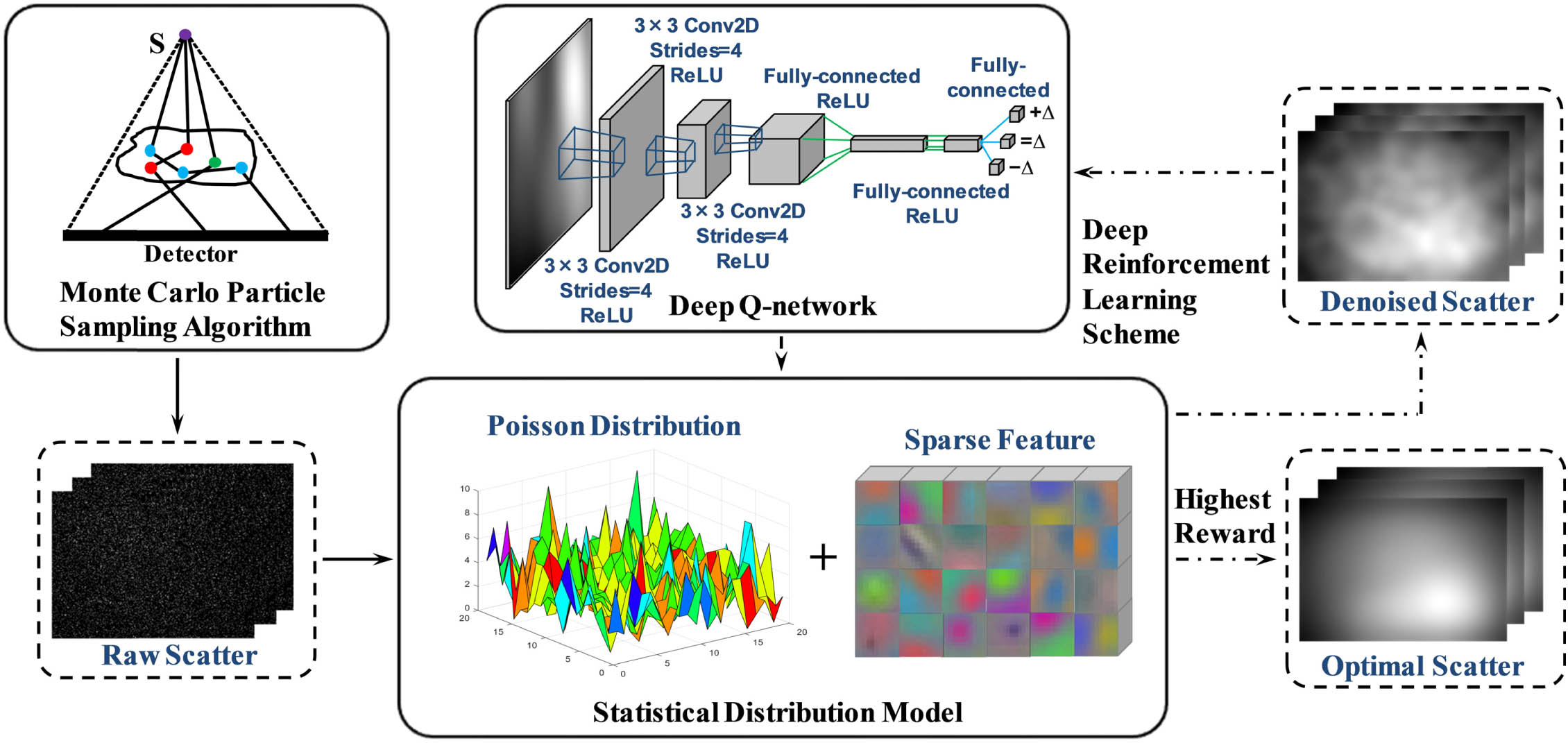
In this study, we propose an ASEF that integrates an MC particle sampling algorithm (details depicted in Section 2.B), a statistical distribution model fused with sparse feature representation under the Poisson distribution assumption (Section 2.C), and a DRL scheme (Section 2.D). The entire framework is illustrated in Fig. 1. First, on the basis of the X-ray source energy spectrum and system geometry configuration, a graphic processing unit (GPU)-based MC simulation initially yields a raw scatter signal with a low photon number to hasten scatter generation. Second, assuming that the scatter signal follows Poisson distribution, an optimization objective function fused with sparse feature penalty is constructed. Then, an over-relaxation algorithm is deduced mathematically to solve this objective function. For optimizing the parameters in the over-relaxation algorithm, a neural network called the deep -network (DQN) is built to intelligently interact with the over-relaxation algorithm for optimal scatter image quality. Specifically, the well trained DQN, which possesses the optimal policy of the highest rewards, takes an action to change the parameters; then the over-relaxation algorithm yields a scatter image based on the adjusted parameters for the next action selection. After several tuning steps, the optimal parameters can be determined when the highest cumulative rewards of a sequence of steps are obtained. The scatter image yielded by the over-relaxation algorithm with the optimal parameters is referred to as optimal quality.
Figure 1.Automatic scatter estimation framework. The MC algorithm generates raw scatter signals in terms of the X-ray source energy spectrum and system geometry configuration. The DRL scheme (denoted by the dashed black arrow) employs a deep -network to interact with the statistical distribution model to yield a satisfactory scatter image.
An in-house MC simulation tool with a polychromatic energy spectrum is utilized in this study for the MC particle sampling of the scatter signal. The energy spectrum describes the probability density of a source photon as a function of its energy. Such an energy spectrum can be specified by using the method developed by Boone et al. [26]. According to tabulated data including the attenuation coefficients and the cross sections of Compton scattering, Rayleigh scattering, and the photoelectric effect, each photon transporting through the imaging phantom is simulated to compute the particle distribution in the virtual detector. During the simulation, an indicator is carried by each photon that records if any scattering events have taken place during the transport. For different scattering events of different orders, the photon will be marked by a number as the indicator of the photon. For example, the indicators of all primal photons are zero, and all first order Compton photons are marked one as the indicator. The CT volume of the phantom is utilized to generate different material and density information on the basis of the CT value via threshold-based segmentation. The MC sampling scheme includes several realistic features, e.g., the polychromatic source spectrum, materials and thicknesses of the detector, and beam collimation.
In the MC particle sampling, the scatter angles for Rayleigh scattering are sampled from the expression for the differential cross sections as and the scatter angles for Compton scattering can be expressed as Note that the photon energy is reduced after the Compton scattering, and is the ratio of the energy before scattering and the current energy : where , , and separately indicate the electron radius, light speed, and resting mass of one electron in Eqs. (1)–(3). The functions and are the form factor and the incoherent scattering function. Data for and are generated from the gCTD package [27], which is a fast MC simulation packge for patient-specific CBCT imaging or dose calculation. For shortening computation time, scatter angles were not sampled by calculating Eqs. (1) and (2) but were taken from the pre-calculated look-up table. Electron transport is neglected in the simulation, as it cannot reach the detector and will be absorbed in the phantom immediately. Moreover, the Woodcock tracking algorithm [28] is employed to avoid calculating the integral of photon path attenuation voxel by voxel.
C. Scatter Statistical Distribution Model Based on Poisson Distribution and Sparse Feature Representation
It has been proved that the measurement determined by the photon distribution statistics follows a Poisson distribution [29,30]. The scatter signal , which is noise-contaminated, is expected to approach true scatter , and thus its probability density function with expectation is defined as where indicates the detector coordinate, for which and denote the horizontal and vertical axes, respectively. Note that measurements are independent of each other, and thus Moreover, Eq. (5) is maximal when , and we minimize rather than maximizing . That is Given the ill-posed nature of Eq. (6), a total-variation (TV) regularization [31] is employed for the smoothness of the solution. Therefore, the formula based on Poisson distribution and sparse feature representation can be defined as follows: where the first data-fidelity term is designed to ensure Poisson distribution, and the second TV regularization term is formulated for noise suppression. is a hyper-parameter controlling the relationship between the data-fidelity and regularization terms. As Eq. (7) is convex, the derivative of its optimal solution is equal to zero, that is, Equation (8) can be discretized as where the Laplacian operator , and stands for . Then, an over-relaxation iteration algorithm is employed to solve Eq. (7): where the superscript represents the iteration step, and is an empirical constant to speed up convergence. Finally, the noise free scatter signal can be obtained by solving Eq. (10) iteratively.
D. Deep Reinforcement Learning
1. Double Deep Q-Network
Three hyper-parameters appear in Eq. (10): , , and the number of iterations to be determined. Typically, these variables are set to a constant to obtain smoothed scatter images even though the simulated photon number is different. Tuning parameters manually for all situations is a trial-and-error process, which calls for considerable time and effort. Moreover, this approach restricts the over-relaxation algorithm from exploring a global optimal solution for improved image quality. These quality-related parameters are not one-size-fits-all for all cases with different photon numbers. Consequently, we aim to utilize a DRL scheme to intelligently seek out satisfactory images like human behavior.
The -learning algorithm is a widely used approach, for which the action-value function is defined as the expectation of the rewards sum of all possible steps from the current state taking action under policy : where is the discounted rewards sum starting from step , is the reward at step , and is a discount factor. The -learning algorithm aims to explore an optimal policy to maximize the action-value function: The optimal action-value function can be solved iteratively via the Bellman equation: where denotes the reward after adopting action to the current state , and is the next state following the current state under action . Equation (14) entails expensive computation when the state and action involve extensive dimensions. Thus, we adopt a convolutional neural network (CNN) to approximate the function , such that a quadratic loss function defined as Eq. (15) can be minimized to force to approach optimal : To enhance the training stability of , a separate target network , whose architecture is the same as the main network , is constructed following the protocol in Ref. [19]. The weights of will be fixed when the main network weight is updated according to the gradient of loss function defined as After several training steps, is updated with ; that is, . The approach based on the -learning algorithm and DNN is referred to as DQN. The DQN tends to over-estimate the action-value function, so we use double DQN (DDQN) for improved robustness [32]. The DDQN utilizes the main network to select the action corresponding to the maximum -value, which is the output value of the network, namely, . Then, action will be utilized in the target network to predict the -value. That is,
2. Reward Function
In DRL, the agent aims to take step-by-step action toward the desired situation by obtaining highest rewards. Therefore, the reward is supposed to faithfully evaluate the quality of state . In this study, state represents the scatter image per angle. Consequently, we employ structural similarity (SSIM) [33] to construct the reward function. The SSIM is a perceptual metric that can quantitatively measure the similarity between two images and , focuses on luminance, contrast, and structure, and is defined as where and separately denote the average of and , and represent variance, and is the covariance of and . A higher SSIM indicates greater similarity between two images. Therefore, the reward function consists of the SSIM of the state and ground truth formulated as where denotes the ground truth of the scatter, and the first and second terms separately measure the SSIM of the scatter at step with the ground truth and the SSIM between the scatter at step and ground truth. will be positive if is closer to the ground truth compared with the previous state , such that it can inspire the DDQN to improve the generated scatter quality toward the desired image quality. sgn indicates the sign function, which transfers a positive number to 1 and a negative number to . As suggested in Ref. [19], the sign function is applied to rescale the reward for the scale limitation of the error derivatives.
3. Training Process of the DDQN
In this study, action has three possible actions: increase or decrease the parameter by 20% and keep it invariant. Some researches [21,23] specified the amount of parameter change with different amplitudes. Because the reward function defined in Eq. (19) utilizes the sign function to restrict the scale of the error derivatives, the network cannot differentiate between rewards of different magnitudes. Therefore, we arbitrarily select 20% as the parameter amplitude. We build our network containing three subnetworks to represent three parameters in the over-relaxation algorithm defined as Eq. (10). These subnetworks possess the same architecture illustrated in Fig. 2. We repeatedly train times, and each episode has a series of steps. At step , one of the three subnetworks is randomly selected with equal probability. Then, the -greedy algorithm is adopted to select an action to adjust the parameter. Specifically, we select a random action with probability ; otherwise, the action corresponding to the highest -value is selected, i.e., . Afterward, the parameter is adjusted according to , and the over-relaxation algorithm is solved to generate a new scatter as the state for the next step. Equation (19) takes and to calculate the reward . The dataset is then stored in the experience replay memory to mitigate the correlation between the training dataset generated in successive steps. Subsequently, network is trained by randomly sampling a mini-batch of dataset from . will be updated via minimizing loss function in Eq. (17). Finally, update target network weights with , i.e., let every steps. The training process of the DDQN is summarized in Table 1, and the related parameter values are defined in Table 2.
Figure 2.Network architecture in the DDQN. The network takes a scatter image as input and predicts three possible actions for parameter adjustment. The number at the top denotes the feature map size and channel number, and the operations for each layer are presented at the bottom. For instance, the first hidden layer convolves 16 filters of with stride four with the input layer followed by a rectified linear unit (ReLU) activation function, and the output layer is a fully connected linear layer with three outputs.
The DDQN can predict an action under the optimal policy. However, the mechanism by which the DDQN takes action in terms of the current state remains unclear. To interpret the DDQN, a gradient-weighted class activation map (Grad-CAM) [34] is utilized to highlight crucial regions in the state for action prediction. The Grad-CAM can yield a localization map using the gradient of output with respect to the last convolution layer to locate regions that are much more important for DDQN decision making. More concretely, Grad-CAM initially calculates the gradient of the -value with respect to the feature map of the last convolutional layer whose width and height are separately indexed by and , namely, . Then, these gradients are backpropagated and global-average-pooled to attain weights for every feature map, i.e., . The Grad-CAM heatmap is the sum of the weighted feature maps and followed by a rectified linear unit (ReLU): . Finally, the Grad-CAM heatmap is upsampled to the input state size.
F. Implementation Details
In this study, we utilize one Nvidia TITAN Xp GPU and four Intel Core i7 3.6 GHz processors with 40 GB memory to implement the framework using TensorFlow [35]. Equation (10) is a noise removal algorithm in the projection domain. Therefore, the scatter is a projection whose resolution is . Six groups of scatter datasets are present with different photon numbers of , , , , , and . Each dataset contains 90 projections. As shown in Fig. 3(i), a raw scatter signal generated from MC simulation with particles is almost noise free and taken as the ground truth. We randomly select 45 of 90 scatter images at for training. The 45 images whose angles differ from those of the training cases in the six groups are chosen as the testing cases. Therefore, the total number of testing cases is 270.
Figure 3.(a) is the primary projection of the head and neck (H&N) patient; (b)–(i) represent raw scatter projections that are separately calculated by the MC particle sampling algorithm with source photons of , , , , , , , and for the same projection angle.
Figures 3(b)–3(i) present the raw scatter signals of the projection produced by the MC particle sampling algorithm with different photon numbers. Figure 3(a) is the primary signal of the projection generated by a typical 100 kVp poly-energetic spectrum with about 100 energy channels. Clearly, Figs. 3(b)–3(h) severely suffer from noise contamination because of the deficiency of source photons (less than ), whereas Fig. 3(i)shows the MC algorithm that can precisely yield a desirable quality scatter image after the photons was simulated. The quantitative evaluation of image similarity and time cost is shown in Tables 3 and 4, respectively. As presented in Table 4, simulating one projection via MC with photons costs 6402.60 s. The computation time of the MC particle sampling algorithm exponentially increases with the growth of the photon number. Therefore, directly producing an approved scatter signal through the MC algorithm would be impractical.
B. Over-Relaxation Smoothing Algorithm for Scatter Estimation
Figures 4(a)–4(g) are the corresponding smoothed scatter signals of Figs. 3(b)–3(h) manipulated by an over-relaxation smoothing algorithm with empirical parameters (, , and ), which is denoted as Empirical for simplicity. The raw scatter projection with photons, as shown in Fig. 4(h), is employed as the ground truth for comparison. The over-relaxation smoothing algorithm can improve scatter image quality among all cases compared to the corresponding raw scatter images. Figures 4(f) and 4(g) are visually similar to Fig. 4(h). Figure 4(e) is slightly rough, whereas Figs. 4(a)–4(d) are severely noisy and fragmentary. The intensity profiles of Figs. 4(a)–4(h) along the row and column indicated by an orange line in Fig. 4(h) are plotted to further validate the performance of the over-relaxation smoothing algorithm. As shown in Figs. 5(a) and 5(b), the intensity profiles of Figs. 4(f) and 4(g) follow exactly the same trend as that in Fig. 4(h). Moreover, the profile lines of Figs. 4(a)–4(e) still oscillate. Therefore, the over-relaxation smoothing algorithm performs well when the photon number is no less than .
Figure 4.(a)–(g) are the scatter images of Figs. 3(b)–3(h) smoothed by the over-relaxation smoothing algorithm; (h) corresponds to Fig. 3(i), which is considered a noise free scatter image and utilized as the ground truth.
To validate its scatter estimation performance, the proposed framework named ASEF is compared with Empirical among six testing groups with dissimilar photon numbers. As depicted in Fig. 6, Empirical alleviates the noise component to some extent but remains inferior compared to ASEF. Although both Empirical and ASEF results degrade as the number of source photons decreases, ASEF scatter images are much more consistent in quality improvement. For the most challenging case with source photons in the first row of Fig. 6, the Empirical scatter image is severely distorted after the over-relaxation smoothing algorithm. By contrast, the ASEF can substantially remove noise and restore the true scatter signal from raw scatter. The ASEF scatter image is visually smoother and similar to the ground truth.
Figure 5.Intensity profiles of Fig. 4 along the (a) horizontal and (b) vertical directions as denoted by the orange lines in Fig. 4(h).
Figure 6.From top to bottom: six testing results with , , , , , and source photons. From left to right: primary signals, smoothed scatter signals restored by the over-relaxation algorithm with empirical parameters, smoothed scatter signals restored by the proposed framework, and the ground truth.
The intensity profiles of Fig. 6 along the vertical direction exhibit the scatter variation trend shown in Fig. 7. Figures 7(a)–7(c) indicate that the ASEF can follow a similar trend to the ground truth, whereas the profile of Empirical oscillates diversely because of the existence of noise. Figure 7(d) suggests that both Empirical and ASEF can obtain satisfactory scatter image quality for the case. However, ASEF possesses a powerful capability of exploring optimal solutions for different source photons (Figs. 6 and 7).
Figure 7.(a)–(d) Intensity profiles of the first, second, third, and last rows in Fig. 6. The locations of the profiles (a)–(d) are denoted by orange lines at the last column of Fig. 6.
For quantitative evaluation, the SSIM, peak signal-to-noise ratio (PSNR), and relative absolute error (RAE) are employed, in which PSNR and RAE are defined as where . MAX denotes the maximum value of scatter signal with dimension .
The SSIM, PSNR, and RAE are treated as three metrics to compare the smoothed scatter results using Empirical and ASEF methods. The result across all testing cases is summarized in Table 3. It is observed that the RAE of ASEF is minimal among all different orders of photon numbers, whereas the SSIM and PSNR are maximal compared to the Empirical method. Table 3 suggests that for the source photons case referred to as the most challenging case in this study, the ASEF can achieve satisfactory performance with , , and . Conversely, the SSIM, PSNR, and RAE of Empirical are 0.79, 21.54 dB, and 12.03%, respectively. The boxplots of the metric difference between Empirical and ASEF are plotted in Figs. 8(a)–8(c). We define metric difference as . Note that the black line in the box denotes the median of difference statistics for each case. In the figure, the absolute value of the difference statistically becomes larger in the SSIM, PSNR, and RAE metrics with the decrease of the source photons. Figure 8(d) shows the SSIM comparison of Empirical and ASEF methods, where it is observed that ASEF is more robust among different photon number cases.
Photon Number
SSIM (1=Best)
PSNR (dB)
RAE (%)
Empirical
ASEF
Empirical
ASEF
Empirical
ASEF
avg.
std.
avg.
std.
avg.
std.
avg.
std.
avg.
std.
avg.
std.
5×10⁵
0.79
4.70×10⁻²
0.94
2.36×10⁻²
21.54
0.85
26.55
1.34
12.03
1.27×10⁻²
5.62
1.27×10⁻²
1×10⁶
0.88
3.73×10⁻²
0.96
1.67×10⁻²
23.99
0.72
29.05
1.22
8.52
9.65×10⁻³
4.22
6.53×10⁻³
5×10⁶
0.97
8.83×10⁻³
0.99
3.85×10⁻³
30.26
0.91
33.76
1.03
3.81
4.69×10⁻³
2.42
3.25×10⁻³
1×10⁷
0.98
4.31×10⁻³
0.99
2.02×10⁻³
33.19
0.83
36.05
0.89
2.68
3.14×10⁻³
1.87
2.35×10⁻³
1×10⁸
0.99
4.96×10⁻⁴
0.99
3.97×10⁻⁴
43.03
0.82
43.96
0.73
0.84
9.31×10⁻⁴
0.74
7.36×10⁻⁴
1×10⁹
0.99
4.84×10⁻⁵
0.99
4.64×10⁻⁵
52.97
0.91
53.12
0.89
0.27
3.26×10⁻⁴
0.26
3.06×10⁻⁴
Table 3. SSIM, PSNR, and RAE Statistics () among All Testing Casesa
Figure 8.(a)–(c) indicate boxplots of the metric difference of SSIM, PSNR, and RAE between Empirical and ASEF for all testing cases. , where metric denotes SSIM, PSNR, and RAE, respectively. (d) is the boxplot of the SSIM comparison of Empirical and ASEF.
To demonstrate the efficiency of the proposed framework, we recorded the computation time of the MC particle sampling algorithm and DRL scheme for one scatter image generation using different photon numbers. MC and DRL are speeded up with one Nvidia TITAN Z GPU with 6 GB memory. Table 4 indicates that the computation burden of the MC algorithm exponentially reduces as the number of photons decrease. The DRL scheme is an interaction process of the neural network and the noise removal algorithm. The computation cost of the neural network is negligible, so the computation time of DRL is dominated by the noise removal algorithm. Note that the DRL process is comprised of a sequence of steps, where the raw scatter with fewer photons takes DRL more steps to find out the optimal parameters. To improve the computational efficiency, the DRL framework is initialized with empirical parameters. When the source photons are no less than , DRL just takes one step to reach the optimal solution, so the computation time of DRL for the last three photon numbers in Table 4 is fixed. Briefly, the overall computation time of the proposed ASEF can be reduced to without loss of quality, an outcome which is extremely fast in the MC simulation domain.
Computation Time (s)
5×10⁵
1×10⁶
5×10⁶
1×10⁷
1×10⁸
1×10⁹
1×10¹⁰
1×10¹¹
MC
0.43
0.45
0.57
0.83
5.94
60.00
633.95
6402.60
DRL
8.98
4.80
1.94
0.98
0.32
0.29
0.29
0.29
Total
9.41
5.25
2.51
1.81
6.26
60.29
634.24
6402.89
Table 4. Computation Time for One Scatter Image of a Prostate Patient across Different Photon Numbers
Figure 9 presents the result during the automatic scatter estimation of the ASEF for a testing case. Figures 9(a)–9(c) are smoothed scatter images at Steps 1, 7, and 13, respectively. Visually, the image quality of the scatter signal is gradually ameliorated with a sequence of tuning steps. This outcome implies that the DDQN has learned an optimal policy to wisely make decisions for parameter adjustment. The SSIM and RAE results over steps are shown in Figs. 9(d) and 9(e). As expected, the SSIM increases step by step, whereas the RAE decreases over steps. Thus, the ASEF can improve scatter image quality intelligently.
Figure 9.Automatic scatter estimation process for a testing case. (a)–(c) are smoothed scatter images at Steps 1, 7, and 13, respectively. (d) and (e) separately plot the SSIM and RAE over steps.
The Grad-CAM heatmaps of the three subnetworks are simultaneously produced when ASEF is verified in the testing case. These heatmaps are upsampled to match the original scatter image size for exhibition and normalized in [0,1], where the prominent region denoted as the red area makes critical contributions to action choice. take the first column of Fig. 10 to predict an action and produce the Grad-CAM heatmaps for each subnetwork shown in the last three columns. The second column is the corresponding ground truth of the first column for visualization comparison. The rows in Fig. 10 represent different scatter images. Note that the high-intensity region of the scatter image in the first row is at the bottom left, whereas the high-intensity area at the third row is close to the image center. The image at the second row has two highlighted regions, for which the major and minor areas are separately located at the bottom and top left. The salient region of the heatmap is approximately located in a high scatter intensity area. The Grad-CAM heatmaps follow a similar scatter intensity distribution of the input state (first column), thereby implying that all three subnetworks consider higher values as crucial features for action prediction. This inference is reasonable because higher scatter intensities are more likely to suffer from noise contamination compared to lower scatter intensity signals.
Figure 10.Different scatter images. From left to right: scatter projection input, the ground truth of the scatter image at the first column, and Grad-CAM heatmaps of three subnetworks .
All of the above training and testing cases are the scatter images of a head and neck (H&N) patient; since the proposed framework can improve image quality dynamically in a manner similar to human intelligence, we utilize scatter images of a prostate patient to further verify it. As depicted by the primary signals in Fig. 11, imaging of the pelvis is so large that it exceeds the field of view (FOV) of a CBCT scan. Thus, the projections of the prostate structure are usually acquired by means of half-fan scanning protocol. It is observed that ASEF is superior compared with Empirical for all prostate cases. Moreover, the intensity profiles of ASEF in Fig. 12 are more similar to the corresponding lines of ground truth, in comparison to the tortuous Empirical lines.
Figure 11.From top to bottom: four prostate cases with , , , and source photons. From left to right: primary signals, smoothed scatter signals restored by the over-relaxation algorithm with empirical parameters, smoothed scatter signals restored by the proposed framework, and the ground truth.
Figure 12.(a)–(d) Intensity profiles of the four prostate cases presented in Fig. 11. Profile locations are outlined by orange lines in the last column of Fig. 11.
As verified in Fig. 3 and Table 4, producing high-quality particle distribution only by the MC algorithm is time-consuming, although the process is speeded up using GPUs. Reducing source photons can considerably improve computational efficiency but lead to noise contamination on the scatter signals. Therefore, an efficient noise removal algorithm based on Poisson distribution and sparse feature fusion is proposed to solve the above issue. The suggested algorithm can effectively make the quality of the scatter signal close to the undistorted signal but degrade gradually for a lower photon number (Figs. 4 and 5). High photon number cases (source photons of over ) can be used for experimental study, which requires good quality at the cost of computation time. Meanwhile, ultra-low photon number cases are applied for clinics since the computation time is considered as a crucial factor in clinics. The DRL scheme is employed to boost the performance of the noise removal algorithm for ultra-low photon number cases. In this way, an automatic scatter estimation scheme suitable for the large range of photon numbers is constructed.
In the study, Figs. 6 and 7 depict the proposed framework that can produce satisfactory scatter signals with different source photons. Table 3 summarizes the results of SSIM, PSNR, and RAE across all testing H&N cases and indicates that ASEF can achieve good performance with , , and . Figure 8 further proves that our framework was robust across different photon numbers. The computational time of ASEF run on the GPU as recorded in Table 4 reveals that our approach is highly efficient with for one scatter projection generation.
The Grad-CAM heatmap was applied to visualize how the DDQN makes action decisions. The region crucial for action prediction is identified in Fig. 10. Obviously, all three subnetworks had conformal intensity distributions similar to the scatter signal, thereby suggesting that the network tends to focus on high scatter intensity areas in view of the fact that the effect of noise on the higher-value region is greater than that in the lower-value counterpart.
We also validated the generalization of the proposed framework on a prostate patient while the DDQN was trained with scatter images of an H&N patient. The scatter signal of prostate patient is much sparser than the H&N scatter signal because the former is acquired by a half-fan scanning protocol. Four prostate scatter projections with , , , and source photons are validated to exhibit the performance. As shown in Fig. 11, the scatter projections by the proposed framework across all cases with different photon numbers were visually superior, and the intensity profiles in Fig. 12 demonstrated the desired performance as well.
With the rapid development of deep-learning algorithms, it is intuitive and straightforward to build end-to-end CNN for scatter removal. Moreover, several researches [36,37] have demonstrated successful applications of this scheme. However, some weaknesses and limitations exist to some extent. Training the CNN requires numerous paired data for which scatter projections calculated by the MC algorithm are generally considered as output labels for supervised learning. As mentioned before, yielding an excellent scatter image with adequate source photons will take substantial time; not to mention, hundreds of scatter projections are required to avoid over-fitting [38]. In addition, scatter signals are highly dependent on the CT geometry configuration and X-ray source energy spectrum [39–42], and the CNN model trained on a dataset may be inappropriate for other types of datasets. Note that only 45 scatter images are used in our DRL training phase. Because of the DRL training strategy illustrated in Table 1, the training datasets stored in the experience replay pool with the capacity of 2000 are rather than 45 images. Furthermore, the training datasets are dynamically updated as the steps change, so there are abundant training data for the neural network model.
5. CONCLUSION
In this study, we proposed an ASEF integrating an MC particle simulation algorithm, statistical distribution model fused with sparse feature representation under Poisson distribution, and a DRL scheme for high-efficiency photon distribution estimation. Experimental results demonstrated that our proposed framework has superior performance for the high-efficiency scatter estimation of large range photon numbers.
Acknowledgment
Acknowledgment. We thank Professor Xun Jia and his MC simulation group from the Department of Radiation Oncology at University of Texas Southwestern Medical Center for their assistance with comments and support on this work.
References
[1] P. J. Verheijen. Statistical distributions in particle technology. Particle Technology Course(2001).
[2] D. A. Nix, A. S. Weigend. Estimating the mean and variance of the target probability distribution. Proceedings of the IEEE International Conference on Neural Networks (ICNN’94), 55-60(1994).
[13] A. Krizhevsky, I. Sutskever, G. E. Hinton. Imagenet classification with deep convolutional neural networks. Advances in Neural Information Processing Systems, 1097-1105(2012).
[14] J. Long, E. Shelhamer, T. Darrell. Fully convolutional networks for semantic segmentation. Proceedings of the IEEE Conference on Computer Vision and Pattern Recognition, 3431-3440(2015).
[15] O. Ronneberger, P. Fischer, T. Brox. U-net: convolutional networks for biomedical image segmentation. International Conference on Medical Image Computing and Computer-Assisted Intervention, 234-241(2015).
[16] K. He, X. Zhang, S. Ren, J. Sun. Deep residual learning for image recognition. Proceedings of the IEEE Conference on Computer Vision and Pattern Recognition, 770-778(2016).
[17] G. Huang, Z. Liu, L. Van Der Maaten, K. Q. Weinberger. Densely connected convolutional networks. Proceedings of the IEEE Conference on Computer Vision and Pattern Recognition, 4700-4708(2017).
[24] C. Shen, L. Chen, Y. Gonzalez, X. Jia. Improving efficiency of training a virtual treatment planner network via knowledge-guided deep reinforcement learning for intelligent automatic treatment planning of radiotherapy(2020).
[28] E. Woodcock, T. Murphy, P. Hemmings, S. Longworth. Techniques used in the GEM code for Monte Carlo neutronics calculations in reactors and other systems of complex geometry. Conference on Applications of Computing Methods to Reactor Problems, 557-579(1965).
[29] E. Jonsson, S. C. Huang, T. Chan. Total variation regularization in positron emission tomography(1998).
[34] R. R. Selvaraju, M. Cogswell, A. Das, R. Vedantam, D. Parikh, D. Batra. Grad-Cam: visual explanations from deep networks via gradient-based localization. Proceedings of the IEEE International Conference on Computer Vision, 618-626(2017).
[35] M. Abadi, P. Barham, J. Chen, Z. Chen, A. Davis, J. Dean, M. Devin, S. Ghemawat, G. Irving, M. Isard. TensorFlow: a system for large-scale machine learning. 12th Symposium on Operating Systems Design and Implementation, 265-283(2016).
[38] N. Srivastava, G. Hinton, A. Krizhevsky, I. Sutskever, R. Salakhutdinov. Dropout: a simple way to prevent neural networks from overfitting. J. Mach. Learn. Res., 15, 1929-1958(2014).