Parallel ray tracing through freeform lenses with NURBS surfaces

Haisong Tang; Zexin Feng; Dewen Cheng; Yongtian Wang

doi:10.3788/COL202321.052201

Journals >Chinese Optics Letters >Volume 21 >Issue 5 >Page 052201 > Article

Chinese Optics Letters
Vol. 21, Issue 5, 052201 (2023)

Parallel ray tracing through freeform lenses with NURBS surfaces

Haisong Tang^1、2, Zexin Feng^1、2、*, Dewen Cheng^1、2, and Yongtian Wang^1、2

Author Affiliations

¹Beijing Engineering Research Center of Mixed Reality and Advanced Display, School of Optics and Photonics, Beijing Institute of Technology, Beijing 100081, China

²MOE Key Laboratory of Optoelectronic Imaging Technology and Systems, Beijing Institute of Technology, Beijing 100081, China

show less

DOI: 10.3788/COL202321.052201 Cite this Article Set citation alerts

Haisong Tang, Zexin Feng, Dewen Cheng, Yongtian Wang. Parallel ray tracing through freeform lenses with NURBS surfaces[J]. Chinese Optics Letters, 2023, 21(5): 052201 Copy Citation Text

EndNote(RIS)

BibTex

Plain Text

show less

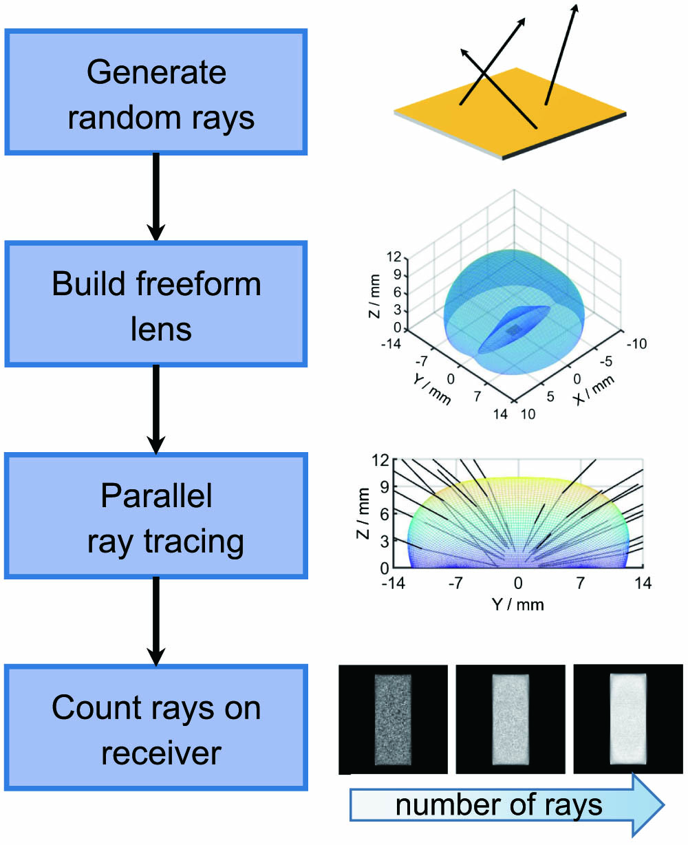
Fig. 1. Flow chart of our parallel ray-tracing algorithm.

Download full size | View in the Article

(a) Zenith angle θ and azimuth angle φ of a randomly sampled ray. (b) The illustration of two different sampling strategies, θ ∼ sin θ and θ ∼ U (0, 0.5π), where φ is uniformly sampled. (c) The distribution of the sampling points with azimuth and zenith angles corresponding to the uniform spatial sampling.

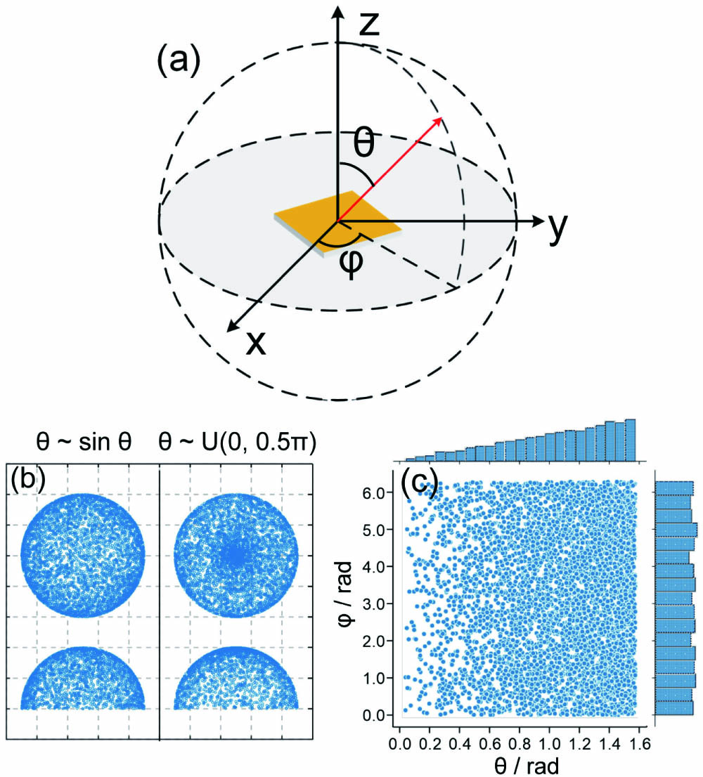
Fig. 2. (a) Zenith angle θ and azimuth angle φ of a randomly sampled ray. (b) The illustration of two different sampling strategies, θ ∼ sin θ and θ ∼ U (0, 0.5π), where φ is uniformly sampled. (c) The distribution of the sampling points with azimuth and zenith angles corresponding to the uniform spatial sampling.

Download full size | View in the Article

$Refraction on freeform surface.$

Fig. 3. Refraction on freeform surface.

Download full size | View in the Article

Fig. 4. Schematic of the ray tracing from the source, through the entrance and exit surfaces of the freeform lens, to the target, generating a complex irradiance pattern.

Download full size | View in the Article

Fig. 5. Illustration of (a) the spherical-freeform lens and an extended light source and (b) the continuous change of the freeform exit surface.

Download full size | View in the Article

Fig. 6. Simulated irradiance distributions of the first example under different settings of the number of rays, the number of cells, and the source size. Each simulated irradiance distribution is in the range of {(x,y) | −1000 mm < x <1000 mm, −1000 mm < y < 1000 mm} and filtered by a 3 × 3 uniform mask.

Download full size | View in the Article

Fig. 7. The second simulation example. (a) The double-freeform lens with a point-like source and (b) its simulation result.

Download full size | View in the Article

Fig. 8. Variations of the runtime with (a) the number of rays, (b) the number of receiver cells, (c) the source size, and (d) the number of control points (of each surface) for the first example.

Download full size | View in the Article

Number of rays		10⁷	10⁶	10⁸	10⁷	10⁷	10⁷	10⁷
Source size		(0.001,0.001)	(0.001,0.001)	(0.001,0.001)	(0.001,0.001)	(0.001,0.001)	(0.001,2.0)	(2.0,2.0)
Number of bins		(128,128)	(128,128)	(128,128)	(64,64)	(256,256)	(128,128)	(128,128)
Time cost (s)		11.16	1.30	112.86	11.13	11.12	11.11	11.17
Intersection precision (mm)	max	2.80 × 10⁻⁴	2.40 × 10⁻⁴	2.83 × 10⁻⁴	2.75 × 10⁻⁴	2.70 × 10⁻⁴	2.72 × 10⁻⁴	2.64 × 10⁻⁴
Intersection precision (mm)	mean	5.33 × 10⁻⁸	5.31 × 10⁻⁸	5.35 × 10⁻⁸	5.33 × 10⁻⁸	5.32 × 10⁻⁸	5.34 × 10⁻⁸	5.34 × 10⁻⁸
Success rate $τ$		0.99978	0.99978	0.99973	0.99978	0.99978	0.99965	0.99945

Table 1. Performances of the Proposed PRT Algorithm Evaluated by the Time Consumption, the Intersection Precision, and the Success Rate τ

View in the Article

Input: length and width of the rectangular light source (

a, b

)

Output: starting points

\hat{s}

, ray directions

\hat{r}

, weights

w

1: function RRS(

a, b

)

σ_{1} \leftarrow RAND ()

σ_{2} \leftarrow RAND ()

σ_{3} \leftarrow RAND ()

σ_{4} \leftarrow RAND ()

x_{0} \leftarrow (σ_{1} - 0.5) a

y_{0} \leftarrow (σ_{2} - 0.5) b

z_{0} \leftarrow 0

θ \leftarrow \arccos (1 - σ_{3})

φ \leftarrow 2 π σ_{4}

r_{x} \leftarrow \sin θ \cos φ

r_{y} \leftarrow \sin θ \sin φ

r_{z} \leftarrow \cos θ

\hat{s} \leftarrow (x_{0}, y_{0}, z_{0}), \hat{r} \leftarrow (r_{x}, r_{y}, r_{z})

w \leftarrow \cos θ

8: return

\hat{s}, \hat{r}, w

9: end function

Table 1. Random rays sampling (RRS) process. The function RAND( ) denotes the generation of a uniformly distributed random number in [0,1]

View in the Article

Input: incident ray parameters

\hat{s}, \hat{r}, w

, surface control points

P

, refractive indices

n_{1}, n_{2}

Output: outgoing ray parameters

{\hat{s}}^{'}, {\hat{r}}^{'}, w^{'}

1: function TRACE(

\hat{s}, \hat{r}, w, P, n_{1}, n_{2}

)

u, v \leftarrow INTER (\hat{s}, \hat{r}, P), \hat{i} \leftarrow \hat{r}

Q, \partial Q / \partial u, \partial Q / \partial v \leftarrow NURBS (u, v, P)

4: get surface normal vectors

\hat{n}

5: get refraction directions

\hat{t}

by Eq. (14)

6: get reflectances

R_{s}

and

R_{p}

based on Eq. (15)

T \leftarrow 1 - (R_{s} + R_{p}) / 2

{\hat{s}}^{'} \leftarrow Q, {\hat{r}}^{'} \leftarrow \hat{t}, w^{'} \leftarrow T \cdot w

9: return

{\hat{s}}^{'}, {\hat{r}}^{'}, w^{'}

10: end function

11: function INTER(

\hat{s}, \hat{r}, P

)

⊳

intersection acquisition

12: generate rough mesh grids

u_{0}, v_{0} \in [0, 1]

13:

A, \partial A / \partial u, \partial A / \partial v \leftarrow NURBS (u_{0}, v_{0}, P)

14:

d \leftarrow 1 - dot (A - \hat{s}, \hat{r}) / {‖ A - \hat{s} ‖}_{2}

15:

d_{\min} = \min (d)

16:

i \leftarrow index (d, d_{\min})

17:

u_{k} \leftarrow u_{0} (i), v_{k} \leftarrow v_{0} (i), d_{k} = d_{\min}

⊳

initial solution

18:

α_{k} \leftarrow - \ln (1 / u_{k} - 1) / 4

β_{k} \leftarrow - \ln (1 / v_{k} - 1) / 4

19: while

d_{k} > ε

⊳

ε

is the allowed error

20:

Q, \partial Q / \partial u, \partial Q / \partial v \leftarrow NURBS (u_{k}, v_{k}, P)

21:

d_{k} \leftarrow 1 - dot (Q - \hat{s}, \hat{r}) / {‖ Q - \hat{s} ‖}_{2}

22: get Jacobian matrix J by Eqs. (9) and (12)

23: get

α_{k + 1}, β_{k + 1}

by Eq. (13)

24:

α_{k} \leftarrow α_{k + 1}, β_{k} \leftarrow β_{k + 1}

25:

u_{k} \leftarrow 1 / (e^{- 4 α_{k}} + 1), v_{k} \leftarrow 1 / (e^{- 4 β_{k}} + 1)

26: end while

27: return

u_{k}, v_{k}

28: end function

29: function NURBS(

u, v, P

)

⊳

surface interpolation

30: generate quasi-uniform node vectors

(u_{1}, u_{2},\dots, u_{i},\dots)

and

(v_{1}, v_{2},\dots, v_{j},\dots)

using shape (

P

)

31: get

N_{i, p} (u), N_{j, q} (v)

based on Eq. (3)

32: get interpolation points

Q

and the partial derivatives

\partial Q / \partial u, \partial Q / \partial v

, while

R_{i, j} = 1

based on Eq. (2)

33: return

Q, \partial Q / \partial u, \partial Q / \partial v

34: end function

Table 2. Light transport simulation through a freeform NURBS surface. During the parallel ray-tracing process, we specify a fixed number of iterations in the INTER( ) function and record the number of rays that satisfy dk≤ε

View in the Article

Input: light source size

(a, b)

, total energy

W_{0}

, number of rays

n

, control points

(P_{1}, P_{2})

of the two surfaces, refractive indices

(n_{1}, n_{2})

of air and lens,

z

-coordinate

z_{r}

of receiver, range

{[x_{\min}, x_{\max}], [y_{\min}, y_{\max}]}

of the receiver, number of cells

(m_{c}, n_{c})

Output: the irradiance distribution on the receiver

E

x_{r} \leftarrow y_{r} \leftarrow w_{r} \leftarrow ZEROS (n)

w_{s} \leftarrow 0

2: for

i = 1

n

{\hat{s}}_{0}, {\hat{r}}_{0}, w_{0} \leftarrow RRS (a, b)

w_{s} \leftarrow w_{s} + w_{0}

{\hat{s}}_{1}, {\hat{r}}_{1}, w_{1} \leftarrow TRACE ({\hat{s}}_{0}, {\hat{r}}_{0}, w_{0}, P_{1}, n_{1}, n_{2})

{\hat{s}}_{2}, {\hat{r}}_{2}, w_{2} \leftarrow TRACE ({\hat{s}}_{1}, {\hat{r}}_{1}, w_{1}, P_{2}, n_{2}, n_{1})

(x, y, z) \leftarrow {\hat{s}}_{2}, (r_{x}, r_{y}, r_{z}) \leftarrow {\hat{r}}_{2}

⊳

decomposition

t \leftarrow (z_{r} - z) / r_{z}

x_{r} (i) \leftarrow x + t \cdot r_{x}, y_{r} (i) \leftarrow y + t \cdot r_{y}, w_{r} (i) \leftarrow w_{2}

10: end for

11:

w_{r} \leftarrow (W_{0} / w_{s}) \cdot w_{r}

12:

E \leftarrow STATIC (x_{r}, y_{r}, w_{r}, m_{c}, n_{c}, x_{\min}, x_{\max}, y_{\min}, y_{\max})

13: function STATIC(

x, y, w, m_{c}, n_{c}, x_{\min}, x_{\max}, y_{\min}, y_{\max}

)

14:

E \leftarrow ZEROS (m_{c}, n_{c})

15: for

i = 1

m_{c}

16: for

j = 1

n_{c}

17:

S_{cell} = (x_{\max} - x_{\min}) \cdot (y_{\max} - y_{\min}) / (m_{c} \cdot n_{c})

18:

w_{i j} \leftarrow

sum

w

of the rays on the

i j

th cell

19:

E_{i j} \leftarrow w_{i j} / S_{cell}

20: end for

21: end for

22: return

E

23: end function

Table 3. Pseudo-code for PRT. We use the GPU to trace batches of light rays simultaneously. The function ZEROS(mc,nc) means generating an mc×nc zeros matrix

Haisong Tang, Zexin Feng, Dewen Cheng, Yongtian Wang. Parallel ray tracing through freeform lenses with NURBS surfaces[J]. Chinese Optics Letters, 2023, 21(5): 052201

Download Citation

EndNote(RIS)

BibTex

Plain Text

Set citation alerts for the article

Tools

Set citation alerts for the article

Save the article for my favorites

Paper Information