Parallel ray tracing through freeform lenses with NURBS surfaces

Haisong Tang; Zexin Feng; Dewen Cheng; Yongtian Wang

doi:10.3788/COL202321.052201

Abstract

We implement Monte Carlo-based parallel ray tracing to achieve quick irradiance evaluation for freeform lenses with non-uniform rational B-splines (NURBS) surfaces. We employ the inverse transform sampling method to sample rays uniformly from the Lambertian light source and adopt the analytical form of the B-spline basis function to achieve fast surface interpolation. When performing parallel calculations for the intersections between the rays and the NURBS surfaces, we propose a parameter transformation method to avoid the parameters escaping from the defined range in the iteration process. Simulation results of two complex picture-generating freeform lenses show that our method is fast and effective.

Keywords

computation methods lenses nonimaging optics propagation methods

1. Introduction

Freeform optics, which refers to refractive or reflective optical elements with freeform surfaces, is considered a revolution in modern optics^[1]. Freeform surfaces are those surfaces that do not have rotational or translational symmetries^[2]. Compared with traditional optical surfaces, including spherical, aspherical, and cylindrical surfaces, freeform surfaces offer much greater design freedom, allowing optical systems to achieve previously unimaginable imaging^[3–5], illumination^[6,7], and laser beam shaping performances^[8]. The performance evaluation of these freeform optical systems is highly dependent on the light transport simulation from source to target. An efficient light transport computation is crucial in finding the optimal freeform optical systems through optimization techniques.

Ray tracing is currently the most popular and powerful technique for light transport simulation. The main operation of ray tracing is to acquire the intersection points between light rays and surfaces. The computation efficiency of this process is strongly influenced by the surface complexities. Freeform surfaces for imaging can be conveniently described by polynomials, e.g., $X Y$ polynomials^[3]. However, plenty of illumination problems, e.g., picture-generating freeform lens design^[6], are solved numerically. The resulting freeform surfaces, which contain many local curvature features, are hard to describe by using polynomial expansions. Time and memory consumption of ray tracing could increase rapidly as the surface representation becomes more and more complex. Generally, iterative methods have to be employed to obtain the intersection points, which heavily rely on the initial solutions. The meshing method is commonly used to find appropriate initial solutions^[9–11]. In this method, the grids are checked one by one to judge if the intersection occurs on the current grid. However, this method becomes less efficient when the required number of mesh grids is large.

Optical surfaces that are highly freeform and contain both global and local structures can be represented by B-splines, especially by its subset, non-uniform rational B-splines (NURBS)^[12,13]. However, it is not easy to determine the intersection points, even their initial approximations, between the rays and the NURBS surface with high efficiency. The clipping method can be employed to accelerate the ray-tracing process of NURBS surfaces^[14,15]. This method adaptively divides the surface parameters into uniform parts on the 2D parameter space to find the region where the light ray intersects with the surface. Then, the region is gradually subdivided to determine an appropriate initial solution. However, this method suffers from reporting wrong intersections because the sampling points on the surface are not uniformly distributed when parameters are uniformly sampled^[15,16].

Sign up for Chinese Optics Letters TOC. Get the latest issue of Chinese Optics Letters delivered right to you！Sign up now

Aside from the intersection problem, another important issue is the way of implementing ray tracing. Although some deterministic methods have been discussed, it is restricted in many applications^[17]. In the evaluation and optimization process, the Monte Carlo (MC) ray-tracing method gains wider acceptance as the gold standard for calculating light transport through optical systems^[18–20]. MC ray tracing randomly samples light rays on a light source with a specific probability and traces the light path through the optical system by Snell’s laws. Then, it accumulates the light energy transmitted to the receiver to calculate the irradiance distribution.

Some commercial softwares can perform MC ray tracing of freeform optical elements and systems, but the related algorithms are rarely discussed publicly. Many self-developed ray-tracing programs are successfully applied to artificial image simulation^[21–27], aberration analysis^[28–32], and optical inspection^[33–36]. Some entire ray-tracing pipelines for nonimaging systems have been described in detail^[11,20]. Most of the current MC ray-tracing algorithms trace rays one by one, based on the same law and formula.

The ray-tracing process could be accelerated if plenty of rays are traced simultaneously. However, it is a high-dimensional problem that the parallel intersection process requires simultaneous acquisition of the initial solutions of all current rays. The traditional way of obtaining an initial solution to the intersection problem of a single ray and the freeform surface requires simultaneous computation on mesh grids, which is not suitable for parallel ray tracing. In addition, when the initial solution is not accurate enough, the parameters of the intersection could easily escape from the defined range as the iteration progresses, resulting in many calculation errors.

We implement MC parallel ray tracing (PRT) for freeform illumination lenses with NURBS surfaces to realize a fast irradiance evaluation. We achieve uniform sampling by inverse transform sampling and fast surface interpolation by adopting the analytical form of the B-spline basis function. We propose a parameter transform method to reduce the accuracy requirement of the initial solution during the intersection process using Newton’s method, which could improve the percentage of successfully traced light rays by parallel computation. This fast MC simulation program can facilitate the evaluation and optimization of freeform lenses. Section 2 describes in detail the parallel ray-tracing method for freeform NURBS surfaces. Section 3 gives two examples to demonstrate the effectiveness of the proposed method.

2. Methods

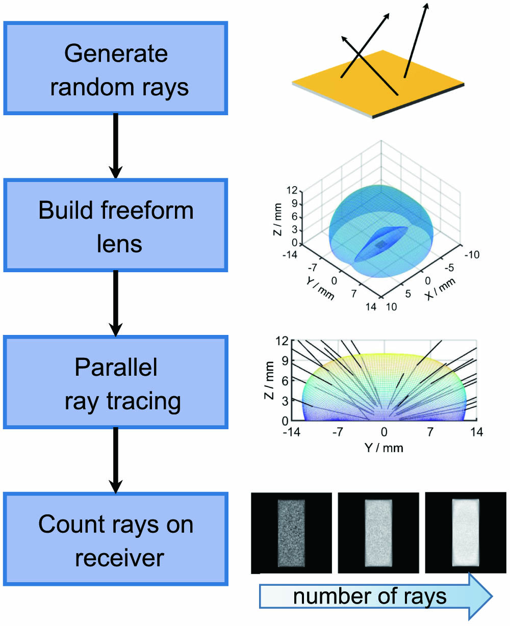
The purpose of the ray-tracing process is to trace the changes in the spatial parameters $(x, y)$ and orientation parameters $(r_{x}, r_{y})$ , which uniquely characterize a light ray in a three-dimensional space. $(x, y, r_{x}, r_{y})$ form a four-dimensional parameter space, which degenerates to a two-dimensional one for a special case when all the rays are emitted from a point light source. Figure 1 illustrates the procedures of our parallel ray-tracing algorithm. After defining the optical system parameters, we sample the light source randomly in both spatial locations and orientations, generating a random set of rays. We then implement MC ray propagation from the source, through the freeform lenses, to the receiver. The difficulty arises in simultaneously determining all the parameters $(x, y, r_{x}, r_{y})$ for the current set of rays transporting through a complex freeform surface. In this decisive and important step, we propose a parameter transformation method to reduce the ray-surface intersection errors in the iterative process of Newton’s method. Finally, we count the number of rays that reach different positions of the receiver to determine the irradiance distribution. The three steps are described in detail in the following section.

Figure 1.Flow chart of our parallel ray-tracing algorithm.

2.1. Sampling rays from the light source

The light source is required to be sampled randomly in both spatial locations and orientations. Different sampling probability density functions $P (x, y, r_{x}, r_{y})$ should ensure that $w (x, y, r_{x}, r_{y}) \cdot P (x, y, r_{x}, r_{y})$ is proportional to $L (x, y, r_{x}, r_{y}) \cdot \cos θ$ , where $L$ is the radiance distribution of the source, $w$ denotes the weights of the sampled rays, and $θ$ denotes the angles from the source surface normal to the sampled rays. The initial values of $w$ can be set as 1, and then $P$ is proportional to the intensity distribution of the light source. However, this can add computation complexity when $L$ is not a constant.

Here, we first sample the position coordinates and solid angle of the light source uniformly and then assign the initial weights proportional to $L \cdot \cos θ$ . In this way, there is an equivalent relation between the radiance distribution $L$ and the weights of the sampled light rays, $L (x, y, r_{x}, r_{y}) \cdot \cos θ δ S δ Ω \propto E_{μ} (\sum_{i = 0}^{k} w_{i}) .$ (1)

Herein, $δ S$ denotes a small area on the surface around $(x, y)$ , and $δ Ω$ denotes a small solid angle around $(x, y, r_{x}, r_{y})$ . $E_{μ} (\sum_{i = 0}^{k} w_{i})$ is the mathematical expectation of the summed weight of the light rays inside the small space $δ S δ Ω$ , and $k$ denotes the number of rays inside the small space.

In a spherical coordinate system, $(r_{x}, r_{y})$ can be replaced with the zenith angle $θ$ and the azimuth angle $φ$ , as shown in Fig. 2(a). Note that the light rays sampled uniformly with $θ$ and $φ$ are not uniformly distributed in space^[19]. Since the magnitude of the small solid angle $δ Ω$ around $(θ, φ)$ is proportional to $\sin θ δ θ δ φ$ , uniform sampling of the solid angle should guarantee that the probability is proportional to $φ$ and $\sin θ$ .

Figure 2.(a) Zenith angle θ and azimuth angle φ of a randomly sampled ray. (b) The illustration of two different sampling strategies, θ ∼ sin θ and θ ∼ U (0, 0.5π), where φ is uniformly sampled. (c) The distribution of the sampling points with azimuth and zenith angles corresponding to the uniform spatial sampling.

We employ the inverse transform sampling method^[37] to obtain random variables with arbitrary probability distribution $f (x)$ , where $x \in [0, 1]$ . This method first calculates the cumulative probability distribution function $F (x) = \int_{- \infty}^{\infty} f (x) d x$ according to the required probability distribution function $f (x)$ . A uniformly distributed random variable $Y = F (x)$ can be generated. Finally, the random variable $X$ with probability distribution $f (X)$ can be obtained as $X = F^{- 1} (x)$ . For the sampling of the zenith angle here, we first obtain a random uniformly distributed variable $Y$ between 0 and 1; then the probability distribution function $X = \arccos (1 - Y)$ is a sine function. Thus, uniform sampling of random rays in space can be generated based on setting the probability distribution functions as $θ \sim \sin θ$ , $φ \sim U (0, 2 π)$ .

Figures 2(b) and 2(c) illustrate the ray distributions of a Lambertian light source sampled in two strategies: $θ \sim \sin θ$ and $θ \sim U (0,0.5 π)$ , where $φ$ is uniformly sampled for each strategy. The pseudo-code of the random rays sampling process is shown in Algorithm 1.

Number of rays		10⁷	10⁶	10⁸	10⁷	10⁷	10⁷	10⁷
Source size		(0.001,0.001)	(0.001,0.001)	(0.001,0.001)	(0.001,0.001)	(0.001,0.001)	(0.001,2.0)	(2.0,2.0)
Number of bins		(128,128)	(128,128)	(128,128)	(64,64)	(256,256)	(128,128)	(128,128)
Time cost (s)		11.16	1.30	112.86	11.13	11.12	11.11	11.17
Intersection precision (mm)	max	2.80 × 10⁻⁴	2.40 × 10⁻⁴	2.83 × 10⁻⁴	2.75 × 10⁻⁴	2.70 × 10⁻⁴	2.72 × 10⁻⁴	2.64 × 10⁻⁴
Intersection precision (mm)	mean	5.33 × 10⁻⁸	5.31 × 10⁻⁸	5.35 × 10⁻⁸	5.33 × 10⁻⁸	5.32 × 10⁻⁸	5.34 × 10⁻⁸	5.34 × 10⁻⁸
Success rate $τ$		0.99978	0.99978	0.99973	0.99978	0.99978	0.99965	0.99945

Table 1. Performances of the Proposed PRT Algorithm Evaluated by the Time Consumption, the Intersection Precision, and the Success Rate τ

View all Tables

2.2. Light propagation through freeform optical surfaces

After generating a sequence of random rays from the light source, we trace the rays propagating through the freeform optical surfaces represented with NURBS. The key operation is the determination of the intersection points between rays and surfaces. Thus, we accelerate the intersection process by modifying the surface interpolation strategy and introducing a parameter transformation method. After obtaining the intersection points, we use Snell’s law in vector form to calculate the outgoing ray vectors.

2.2.1. Intersection acquisition on optical surface

An NURBS surface is obtained as the tensor product of two NURBS curves parameterized by two parameters $u$ and $v$ , $Q (u, v) = \sum_{i = 0}^{m_{s} - 1} \sum_{j = 0}^{n_{s} - 1} N_{i, p} (u) N_{j, q} (v) R_{i, j} P (i, j),$ (2)where $u$ and $v$ lie in $[0, 1]$ , $P (i, j)$ denotes the control point, $R_{i, j}$ is the weight of $P (i, j)$ , and $N_{i, p} (u)$ and $N_{j, q} (v)$ are the basis functions of the B-splines of degree $p$ and $q$ in the $u$ and $v$ directions, respectively. The basis function $N_{i, p} (u)$ is defined by the De Boor Cox recursion formula^[12], ${\begin{cases} N_{i,0} = {\begin{cases} 1 & if u \in [u_{i}, u_{i + 1}) \\ 0 & if else \end{cases}, \\ N_{i, p} = \frac{u - u_{i}}{u_{i + p} - u_{i}} N_{i, p - 1} (u) + \frac{u_{i + p + 1} - u}{u_{i + p + 1} - u_{i + 1}} N_{i + 1, p - 1} (u), \\ define: \frac{0}{0} = 0 . \end{cases}$ (3)

Herein, $u_{i}$ is the selected node which divides $[0, 1]$ into $m_{s} + p$ segments. We employ the quasi-uniform nodes here, which can simplify the formula for the B-spline basis functions.

The computation volume required for interpolation increases exponentially with the number of control points and the interpolation degree. The major reason is that the recursive method repeatedly computes the formula with a large storage of accumulative data and no zero $N (u_{i})$ only when $u_{i} \in [u_{i}, u_{i + p + 1}]$ . These unnecessary calculations slow down the intersection point-finding process. Abert et al. transferred the computationally expensive recursion into single instruction multiple-data (SIMD) suitable form to reduce the time cost of executed commands^[13]. Jester et al. proposed the B-spline quasi-interpolation scheme, which improves the computational speed of B-spline surfaces within a certain error range^[38]. To improve the speed of the interpolation process, we employ the analytical form of the B-spline basis function of degree 2^[13]. In addition, only the control points whose corresponding basis functions are not 0 are considered in the interpolation process to avoid meaningless operations. Such a strategy can promote calculation efficiency greatly when the control point number is much larger than the interpolation order.

After specifying the interpolation strategy, let us now turn to the calculation of the intersection between the rays and the NURBS surface. Suppose we have a ray parameterized as $(x (t), y (t), z (t)) = \hat{s} + \hat{r} \cdot t$ , where $\hat{s} = (x_{0}, y_{0}, z_{0})$ is the starting point, and $\hat{r} = (r_{x}, r_{y}, r_{z})$ denotes the ray direction. The intersection can be formulated by the following equation: $Q (u, v) = \hat{s} + \hat{r} \cdot t,$ (4)where $Q = (Q_{1}, Q_{2}, Q_{3})$ denotes a point on the NURBS surface. After expressing the ray direction with $θ$ and $φ$ , Eq. (4) can be rewritten as ${\begin{cases} Q_{1} (u, v) - x_{0} = \sin θ \cos φ \cdot t \\ Q_{2} (u, v) - y_{0} = \sin θ \sin φ \cdot t \\ Q_{3} (u, v) - z_{0} = \cos θ \cdot t \end{cases} .$ (5)

We rotate $φ$ and $θ$ around the $z$ -axis and $y$ -axis, respectively, so that the new $z$ -axis coincides with the direction of the light ray. This way can simplify the intersection-solving process^[39]. The transformation matrices describing the rotations are $R_{z} = [\begin{matrix} \cos φ & \sin φ & 0 \\ - \sin φ & \cos φ & 0 \\ 0 & 0 & 1 \end{matrix}], R_{y} = [\begin{matrix} \cos θ & 0 & - \sin θ \\ 0 & 1 & 0 \\ \sin θ & 0 & \cos θ \end{matrix}],$ (6)where $R_{z}$ describes the rotation around the $z$ -axis, and $R_{y}$ describes the rotation around the $y$ -axis.

After applying the rotation matrices to Eq. (5), we obtain $R_{y} \cdot R_{z} \cdot [\begin{matrix} Q_{x} (u, v) - x_{0} \\ Q_{y} (u, v) - y_{0} \\ Q_{z} (u, v) - z_{0} \end{matrix}] = R_{y} \cdot R_{z} \cdot [\begin{matrix} \sin θ \cdot \cos φ \cdot t \\ \sin θ \cdot \sin φ \cdot t \\ \cos θ \cdot t \end{matrix}] = [\begin{matrix} 0 \\ 0 \\ t \end{matrix}] .$ (7)

We take the first two equations, which could be represented as $f_{1} (u, v) = 0 and f_{2} (u, v) = 0$ . Then, the parameters $(u, v)$ of the intersection point on the surface can be solved by using Newton’s method. Newton’s iteration step is given by $[\begin{matrix} u_{k + 1} \\ v_{k + 1} \end{matrix}] = [\begin{matrix} u_{k} \\ v_{k} \end{matrix}] - J^{- 1} [\begin{matrix} f_{1} (u_{k}, v_{k}) \\ f_{2} (u_{k}, v_{k}) \end{matrix}],$ (8)where $(u_{k}, v_{k})$ is the approximate solution of the $k$ th iteration, and J is the Jacobian matrix, $J = [\begin{matrix} \frac{\partial f_{1}}{\partial u} & \frac{\partial f_{1}}{\partial v} \\ \frac{\partial f_{2}}{\partial u} & \frac{\partial f_{2}}{\partial v} \end{matrix}] .$ (9)

Newton’s method needs a good initial estimate. Most of the methods divide the surface into many triangular meshes to find a suitable initial solution. If the meshing is sufficiently detailed, then the initial solution could lead to a good iteration result. Such a strategy is not suitable for parallel computation here.

A slight deviation from the exact initial solution could cause the value of $u$ or $v$ to exceed the range of [0,1], resulting in surface interpolation errors. We adopt a parameter transformation method to solve this problem. In this method, a new pair of parameters, $(α, β)$ , are employed to replace $(u, v)$ , and their relationships can be described as $u = \frac{1}{e^{- 4 α} + 1}, v = \frac{1}{e^{- 4 β} + 1} .$ (10)

The parameter transformation has the following characteristics: ${\begin{cases} α, β \in (- \infty, + \infty), u, v \in (0, 1) \\ \frac{d u}{d α} > 0, \frac{d v}{d β} > 0, {\frac{d u}{d α} |}_{α = 0} = 1, {\frac{d v}{d β} |}_{β = 0} = 1 \\ {u |}_{α = 0} = 0.5, {v |}_{β = 0} = 0.5 \end{cases} .$ (11)

Such a transformation can avoid the values of $(u, v)$ exceeding [0, 1]. The intersection equations now become $f_{1} (α, β) = 0 and f_{2} (α, β) = 0$ . The new Jacobian matrix J in Newton’s method can be acquired based on the chain rule ${\begin{matrix} \frac{\partial f}{\partial α} & = & \frac{\partial f}{\partial u} \cdot \frac{d u}{d α} \\ \frac{\partial f}{\partial β} & = & \frac{\partial f}{\partial v} \cdot \frac{d v}{d β} \end{matrix} .$ (12)

Herein, $f$ can be $f_{1}$ or $f_{2}$ . We obtain the initial solution using a coarse mesh on the surface. For the $k$ th iteration, $(α_{k}, β_{k})$ can be calculated from $(u_{k}, v_{k})$ by the inverse operation of Eq. (10). The Newton iteration formula Eq. (8) is changed into $[\begin{matrix} α_{k + 1} \\ β_{k + 1} \end{matrix}] = [\begin{matrix} α_{k} \\ β_{k} \end{matrix}] - J^{- 1} [\begin{matrix} f_{1} (α_{k}, β_{k}) \\ f_{2} (α_{k}, β_{k}) \end{matrix}] .$ (13)

Such a parameter transformation could reduce the accuracy requirement of the initial solution to the iterative computation. Thus, we can adopt surface points with a relatively coarse density as the initial solution, which can save a lot of time.

2.2.2. Refraction on the optical surface

Once we obtain the intersection points between the rays and the surface, we determine the refraction directions of the outgoing rays based on Snell’s law. As illustrated in Fig. 3, $\hat{i}$ denotes the unit incident ray vectors, $\hat{t}$ denotes the unit outgoing ray vectors, $\hat{n}$ denotes the unit normal vectors to the intersection points on the surface, and $n_{1}$ and $n_{2}$ denote the refractive indices of the incident and exit media. Then, $\hat{t}$ can be obtained based on Snell’s law in vector form, $\hat{t} = \frac{1}{n_{2}} {n_{1} \hat{i} + [\sqrt{n_{2}^{2} - n_{1}^{2} + n_{1}^{2} {(\hat{n} \cdot \hat{i})}^{2}} - n_{1} \hat{n} \cdot \hat{i}] \hat{n}} .$ (14)

$Refraction on freeform surface.$

Figure 3.Refraction on freeform surface.

Fresnel loss occurs when a light ray passes through a refractive optical surface. The reflectivities $r_{s}$ and $r_{p}$ for s-polarized light and p-polarized light, respectively, are written as $r_{s} = \frac{n_{1} \cos θ_{i} - n_{2} \cos θ_{t}}{n_{1} \cos θ_{i} + n_{2} \cos θ_{t}}, r_{p} = \frac{n_{1} \cos θ_{t} - n_{2} \cos θ_{i}}{n_{1} \cos θ_{t} + n_{2} \cos θ_{i}},$ (15)where $θ_{i}$ and $θ_{t}$ denote the incident and refracted angles, respectively. The reflectances $R_{s}$ and $R_{p}$ for s-polarized light and p-polarized light, respectively, can be obtained as $R_{s} = r_{s}^{2} and R_{p} = r_{p}^{2}$ . The transmittances $T_{s}$ and $T_{p}$ for s-polarized light and p-polarized light, respectively, can be simply obtained as $T_{s} = 1 - R_{s}$ and $T_{p} = 1 - R_{p}$ . For natural light or typical LED light, the total transmittance $T$ can be taken as the average of $T_{s}$ and $T_{p}$ . We adjust the weights $w (x, y, r_{x}, r_{y})$ of the light rays according to the transmittance $T$ during ray tracing.

The pseudo-code for simulating the light transport through a freeform surface is provided in Algorithm 2. Herein, we consider ray tracing as successful when the cosine distance $d = 1 - dot (Q - \hat{s}, \hat{r}) / {‖ Q - \hat{s} ‖}_{2}$ is less than the allowed error $ε$ , where Q is the found intersection point.

Input: incident ray parameters

\hat{s}, \hat{r}, w

, surface control points

P

, refractive indices

n_{1}, n_{2}

Output: outgoing ray parameters

{\hat{s}}^{'}, {\hat{r}}^{'}, w^{'}

1: function TRACE(

\hat{s}, \hat{r}, w, P, n_{1}, n_{2}

)

u, v \leftarrow INTER (\hat{s}, \hat{r}, P), \hat{i} \leftarrow \hat{r}

Q, \partial Q / \partial u, \partial Q / \partial v \leftarrow NURBS (u, v, P)

4: get surface normal vectors

\hat{n}

5: get refraction directions

\hat{t}

by Eq. (14)

6: get reflectances

R_{s}

and

R_{p}

based on Eq. (15)

T \leftarrow 1 - (R_{s} + R_{p}) / 2

{\hat{s}}^{'} \leftarrow Q, {\hat{r}}^{'} \leftarrow \hat{t}, w^{'} \leftarrow T \cdot w

9: return

{\hat{s}}^{'}, {\hat{r}}^{'}, w^{'}

10: end function

11: function INTER(

\hat{s}, \hat{r}, P

)

⊳

intersection acquisition

12: generate rough mesh grids

u_{0}, v_{0} \in [0, 1]

13:

A, \partial A / \partial u, \partial A / \partial v \leftarrow NURBS (u_{0}, v_{0}, P)

14:

d \leftarrow 1 - dot (A - \hat{s}, \hat{r}) / {‖ A - \hat{s} ‖}_{2}

15:

d_{\min} = \min (d)

16:

i \leftarrow index (d, d_{\min})

17:

u_{k} \leftarrow u_{0} (i), v_{k} \leftarrow v_{0} (i), d_{k} = d_{\min}

⊳

initial solution

18:

α_{k} \leftarrow - \ln (1 / u_{k} - 1) / 4

β_{k} \leftarrow - \ln (1 / v_{k} - 1) / 4

19: while

d_{k} > ε

⊳

ε

is the allowed error

20:

Q, \partial Q / \partial u, \partial Q / \partial v \leftarrow NURBS (u_{k}, v_{k}, P)

21:

d_{k} \leftarrow 1 - dot (Q - \hat{s}, \hat{r}) / {‖ Q - \hat{s} ‖}_{2}

22: get Jacobian matrix J by Eqs. (9) and (12)

23: get

α_{k + 1}, β_{k + 1}

by Eq. (13)

24:

α_{k} \leftarrow α_{k + 1}, β_{k} \leftarrow β_{k + 1}

25:

u_{k} \leftarrow 1 / (e^{- 4 α_{k}} + 1), v_{k} \leftarrow 1 / (e^{- 4 β_{k}} + 1)

26: end while

27: return

u_{k}, v_{k}

28: end function

29: function NURBS(

u, v, P

)

⊳

surface interpolation

30: generate quasi-uniform node vectors

(u_{1}, u_{2},\dots, u_{i},\dots)

and

(v_{1}, v_{2},\dots, v_{j},\dots)

using shape (

P

)

31: get

N_{i, p} (u), N_{j, q} (v)

based on Eq. (3)

32: get interpolation points

Q

and the partial derivatives

\partial Q / \partial u, \partial Q / \partial v

, while

R_{i, j} = 1

based on Eq. (2)

33: return

Q, \partial Q / \partial u, \partial Q / \partial v

34: end function

Table 2. Light transport simulation through a freeform NURBS surface. During the parallel ray-tracing process, we specify a fixed number of iterations in the INTER( ) function and record the number of rays that satisfy $d_{k} \leq ε$

View all Tables

After finishing the ray tracing through the entrance surface, the ray tracing through the second surface can be implemented based on the same procedure, where the intersection points on the entrance surface are set as the starting points of the next ray tracing. Such a process is repeated until the light rays hit the receiver.

2.3. Energy statistics on the receiver

After finishing the ray tracing through all the freeform surfaces and determining the intersection points between the rays and the target plane, we count the number of rays for each small grid of the discretized receiver.

Suppose that the total radiant power emitted from the light source is $W_{0}$ . The weight of the $i$ th ray is denoted as $w_{0, i}$ , and the number of rays is $n$ . The radiant power of a ray with the unit weight can be acquired by $W_{unit} = \frac{W_{0}}{\sum_{i = 1}^{n} w_{0, i}} .$ (16)

Suppose that the range of the receiver is ${(x, y) | x_{\min} < x < x_{\max}, y_{\min} < y < y_{\max}}$ , which is discretized into $m_{c} \times n_{c}$ cells. The area of each cell can be obtained as $S_{cell} = \frac{(x_{\max} - x_{\min}) \cdot (y_{\max} - y_{\min})}{m_{c} \cdot n_{c}} .$ (17)

The energy weight of the $i$ th light ray that hits the receiver is changed into $w_{i^{'}}$ . The total number of rays of the $j$ th cell is $n_{j}$ . The irradiance value of the $j$ th cell, $j = 1, 2, \dots$ , $m_{c} \times n_{c}$ , can be acquired by $E_{j} = \frac{W_{unit} \times \sum_{i = 1}^{n_{j}} w_{i^{'}}}{S_{cell}} .$ (18)

The pseudo-code of the energy statistic process and the arithmetic flow of our PRT are shown in Algorithm 3. Note that the more the total traced rays, the higher the signal-to-noise ratio (SNR) of the simulated irradiance distribution. A discussion of the appropriate number of rays to be traced for a certain setting can be found in Ref. [40].

Input: light source size

(a, b)

, total energy

W_{0}

, number of rays

n

, control points

(P_{1}, P_{2})

of the two surfaces, refractive indices

(n_{1}, n_{2})

of air and lens,

z

-coordinate

z_{r}

of receiver, range

{[x_{\min}, x_{\max}], [y_{\min}, y_{\max}]}

of the receiver, number of cells

(m_{c}, n_{c})

Output: the irradiance distribution on the receiver

E

x_{r} \leftarrow y_{r} \leftarrow w_{r} \leftarrow ZEROS (n)

w_{s} \leftarrow 0

2: for

i = 1

n

{\hat{s}}_{0}, {\hat{r}}_{0}, w_{0} \leftarrow RRS (a, b)

w_{s} \leftarrow w_{s} + w_{0}

{\hat{s}}_{1}, {\hat{r}}_{1}, w_{1} \leftarrow TRACE ({\hat{s}}_{0}, {\hat{r}}_{0}, w_{0}, P_{1}, n_{1}, n_{2})

{\hat{s}}_{2}, {\hat{r}}_{2}, w_{2} \leftarrow TRACE ({\hat{s}}_{1}, {\hat{r}}_{1}, w_{1}, P_{2}, n_{2}, n_{1})

(x, y, z) \leftarrow {\hat{s}}_{2}, (r_{x}, r_{y}, r_{z}) \leftarrow {\hat{r}}_{2}

⊳

decomposition

t \leftarrow (z_{r} - z) / r_{z}

x_{r} (i) \leftarrow x + t \cdot r_{x}, y_{r} (i) \leftarrow y + t \cdot r_{y}, w_{r} (i) \leftarrow w_{2}

10: end for

11:

w_{r} \leftarrow (W_{0} / w_{s}) \cdot w_{r}

12:

E \leftarrow STATIC (x_{r}, y_{r}, w_{r}, m_{c}, n_{c}, x_{\min}, x_{\max}, y_{\min}, y_{\max})

13: function STATIC(

x, y, w, m_{c}, n_{c}, x_{\min}, x_{\max}, y_{\min}, y_{\max}

)

14:

E \leftarrow ZEROS (m_{c}, n_{c})

15: for

i = 1

m_{c}

16: for

j = 1

n_{c}

17:

S_{cell} = (x_{\max} - x_{\min}) \cdot (y_{\max} - y_{\min}) / (m_{c} \cdot n_{c})

18:

w_{i j} \leftarrow

sum

w

of the rays on the

i j

th cell

19:

E_{i j} \leftarrow w_{i j} / S_{cell}

20: end for

21: end for

22: return

E

23: end function

Table 3. Pseudo-code for PRT. We use the GPU to trace batches of light rays simultaneously. The function $ZEROS (m_{c}, n_{c})$ means generating an $m_{c} \times n_{c}$ zeros matrix

View all Tables

3. Results

To demonstrate the effectiveness of our method, we implement irradiance evaluation of the picture-generating freeform lenses designed with the iterative wavefront tailoring (IWT) method^[41]. As shown in Fig. 4, the light rays emitted from a light source propagate through the entrance and exit optical surfaces and then generate a complex irradiance distribution of the picture type at the receiver. The entrance surface can be a spherical, aspherical, or freeform surface, and the exit surface is a freeform one. Note that the freeform surface profiles of the picture-generating freeform lenses can be very complex, which is difficult to be described by conventional polynomials, e.g., $X Y$ or Zernike polynomials.

Figure 4.Schematic of the ray tracing from the source, through the entrance and exit surfaces of the freeform lens, to the target, generating a complex irradiance pattern.

The ray tracing performances are evaluated by the time consumption, the intersection precision, and the success rate. The intersection precision is measured by the maximum or average value of the Euclidean distances from the calculated intersection points on the exit surface to the light rays. The success rate $τ$ is defined as the ratio of the number of successfully traced rays to the total number of traced rays.

Our computer is equipped with an Intel i9-12900 k CPU with x86-64 architecture and an NVIDIA RTX3090 GPU with 24 GB video memory and NVIDIA Ampere architecture. The programming language is Python 3.11. We use the GPU to trace batches of light rays simultaneously and the CPU to control the calculation flow. We use the CuPy package of Python for surface modeling, intersection solving, and other parallel scientific calculations. The computing time is mainly affected by the GPU performance.

The first example is the ray tracing of a spherical-freeform lens as shown in Fig. 5(a). The refractive index of the lens is 1.4932. This lens is aimed at converting the light distribution of an LED source into a $2000 mm \times 2000 mm$ irradiance distribution at $z = 1000 mm$ , forming the letters “BIT”. The maximum dimensions of the lens along the $x$ , $y$ , and $z$ directions are 16.97 mm, 16.28 mm, and 12.01 mm, respectively. It can be seen from Fig. 5(b) that the freeform exit surface has complex local features which are directly related to the target irradiance pattern. The entrance surface is $50 \times 50$ 3D grids sampled from a semi-sphere of 5 mm radius, which is also expressed with NURBS. The complex exit freeform surface is described by $256 \times 256$ control points. We employ a $3 \times 3$ uniform filter for the simulated irradiance distribution to decrease the noise of the MC method. Figure 6 shows the simulated irradiance distributions of our algorithm under different settings of the number of light rays $n$ , the number of receiver cells $m = m_{c} \times n_{c}$ , and the source sizes. Table 1 gives the corresponding time consumption, precision of the solved intersections, and the success rates.

Figure 5.Illustration of (a) the spherical-freeform lens and an extended light source and (b) the continuous change of the freeform exit surface.

Figure 6.Simulated irradiance distributions of the first example under different settings of the number of rays, the number of cells, and the source size. Each simulated irradiance distribution is in the range of {(x,y) | −1000 mm < x <1000 mm, −1000 mm < y < 1000 mm} and filtered by a 3 × 3 uniform mask.

Number of rays		10⁷	10⁶	10⁸	10⁷	10⁷	10⁷	10⁷
Source size		(0.001,0.001)	(0.001,0.001)	(0.001,0.001)	(0.001,0.001)	(0.001,0.001)	(0.001,2.0)	(2.0,2.0)
Number of bins		(128,128)	(128,128)	(128,128)	(64,64)	(256,256)	(128,128)	(128,128)
Time cost (s)		11.16	1.30	112.86	11.13	11.12	11.11	11.17
Intersection precision (mm)	max	2.80 × 10⁻⁴	2.40 × 10⁻⁴	2.83 × 10⁻⁴	2.75 × 10⁻⁴	2.70 × 10⁻⁴	2.72 × 10⁻⁴	2.64 × 10⁻⁴
Intersection precision (mm)	mean	5.33 × 10⁻⁸	5.31 × 10⁻⁸	5.35 × 10⁻⁸	5.33 × 10⁻⁸	5.32 × 10⁻⁸	5.34 × 10⁻⁸	5.34 × 10⁻⁸
Success rate $τ$		0.99978	0.99978	0.99973	0.99978	0.99978	0.99965	0.99945

Table 1. Performances of the Proposed PRT Algorithm Evaluated by the Time Consumption, the Intersection Precision, and the Success Rate τ

View all Tables

As shown in Table 1, for each case of the first example, the success rate $τ$ is higher than 99.9%. $τ$ could be reduced to below about 96% without using the parameter transformation method. In addition, the parameter transformation method improves the convergence of Newton’s method for solving the intersection points. The iterative solutions would not jump out of the allowed range of the parameters in the early stage of the iterative process. However, the intersection calculation errors can rise rapidly toward the edge of the surface ( $u, v \to 0$ or 1) since the derivatives $(d α / d u, d β / d v)$ of the transformation functions tend to 0. This problem could be avoided by extending the surface so that the active area is bounded away from the edge of the surface.

The second example is about the ray tracing of a more complex double-freeform lens with the maximum dimensions of $15.33 mm \times 16.47 mm \times 10.04 mm$ [see Fig. 7(a)], whose refractive index is also 1.4932. Each of the freeform surfaces contains $1024 \times 1024$ control points. This freeform lens aims at generating a portrait of Johann Carl Friedrich Gauss^[42] with the size of $240 mm \times 240 mm$ at $z = 100 mm$ from a point-like source whose size is $0.001 mm \times 0.001 mm$ . We perform the PRT using $10^{7}$ rays. The simulated irradiance distribution is shown in Fig. 7(b). The maximum and average values of the distances from the calculated intersection points on the exit surface to the light rays are $2.33 \times 10^{- 7} mm$ and $5.16 \times 10^{- 8} mm$ , respectively. Our program only takes $\sim 11.52 s$ to perform the simulation, and $τ$ is about 99.951%.

Figure 7.The second simulation example. (a) The double-freeform lens with a point-like source and (b) its simulation result.

We analyze the time complexity of our PRT program for the first example with respect to the number of rays, the number of receiver cells, the size of the light source, and the number of control points. We use the control variable method to practically test the time consumption of the program. The results are presented in Fig. 8. The time complexity for the number of rays is $O (n)$ . Because $n$ is much larger than the number of GPU cores, parallel computing is still done in batches on the hardware. As shown in Fig. 8(a), the simulation time increases linearly as $n$ increases. For the number of receiver cells, the total time complexity is approximately $O (1)$ . As shown in Fig. 8(b), as $m$ increases, the simulation time remains almost unchanged. The reason is that most of the time is spent on the intersection-seeking process. Theoretically, the time complexity of the ray energy statistical process is $O (m)$ . However, since $n$ is typically much larger than $m$ to ensure low-level Monte Carlo noise, the impact of $m$ on the overall simulation time is negligible. The total time complexity for the source size is about $O (1)$ , as illustrated in Fig. 8(c). The source size only affects the range of the starting points of the randomly sampled rays. We adopt the 2-order analytic form of the NURBS basis functions, which can avoid many recursive operations in base function modeling. Thus, the total time complexity for the control points of the lens surfaces is $O (1)$ , as demonstrated in Fig. 8(d).

Figure 8.Variations of the runtime with (a) the number of rays, (b) the number of receiver cells, (c) the source size, and (d) the number of control points (of each surface) for the first example.

4. Conclusion and Discussion

We have proposed a PRT method for freeform lenses with complex NURBS surfaces. In this method, we employ the inverse transform sampling strategy to uniformly sample rays in space. We also adopt the analytical form of the B-spline basis function of 2 degrees to achieve a fast surface interpolation. More importantly, we proposed a parameter transform method to reduce the initial solution requirement of Newton’s method for solving intersections, which thus increases the success rate of parallel ray tracing. Two examples verify that the proposed PRT method is efficient and effective for quick irradiance evaluations of complex freeform irradiance tailoring lenses.

The proposed PRT method is also applicable to freeform surfaces with other expressions, including $X Y$ polynomials, Zernike polynomials, and radial base functions. Our method can help designers quickly evaluate their design results, especially for freeform surfaces with high degrees of freedom. As a relatively fast irradiance evaluation technique, our method can also be applied to the optimal design of freeform lenses. The proposed method is currently restricted to those cases in which a single light ray does not have multiple intersections with a surface. However, such a restriction is fulfilled by most of the freeform lens designs for illumination and beam-shaping applications. Future work may include the development of non-sequential PRT algorithms and the application of freeform illumination lens design using the automatic differentiation technique in the framework of MindSpore.

References

[1] S. Wills. Freeform optics: notes from the revolution. Opt. Photon. News, 28, 34(2017).

[2] K. Garrard, T. Bruegge, J. Hoffman, T. Dow, A. Sohn. Design tools for freeform optics. Proc. SPIE, 5874, 58740A(2005).

[3] J. P. Rolland, M. A. Davies, T. J. Suleski, C. Evans, A. Bauer, J. C. Lambropoulos, K. Falaggis. Freeform optics for imaging. Optica, 8, 161(2021).

[4] S. Mao, Y. Li, J. Jiang, S. Shen, K. Liu, M. Zheng. Design of a hyper-numerical-aperture deep ultraviolet lithography objective with freeform surfaces. Chin. Opt. Lett., 16, 030801(2018).

[5] D. Cheng, H. Chen, T. Yang, J. Ke, Y. Li, Y. Wang. Optical design of a compact and high-transmittance compressive sensing imaging system enabled by freeform optics. Chin. Opt. Lett., 19, 112202(2021).

[6] R. Wu, Z. Feng, Z. Zheng, R. Liang, P. Benítez, J. C. Miñano, F. Duerr. Design of freeform illumination optics. Laser Photonics Rev., 12, 1700310(2018).

[7] Z. Feng, D. Cheng, Y. Wang. Iterative freeform lens design for prescribed irradiance on curved target. Opto-Electron. Adv., 3, 200010(2020).

[8] Z. Feng, D. Cheng, Y. Wang. Iterative freeform lens design for optical field control. Photon. Res., 9, 1775(2021).

[9] S. Ortiz, D. Siedlecki, L. Remón, S. Marcos. Three-dimensional ray tracing on Delaunay-based reconstructed surfaces. Appl. Opt., 48, 3886(2009).

[10] S. Schedin, P. Hallberg, A. Behndig. Three-dimensional ray-tracing model for the study of advanced refractive errors in keratoconus. Appl. Opt., 55, 507(2016).

[11] R. Kimura. Accelerated ray tracing for headlamp simulation(2017).

[12] J. Ye, L. Chen, X. Li, Q. Yuan, Z. Gao. Review of optical freeform surface representation technique and its application. Opt. Eng., 56, 110901(2017).

[13] O. Abert, M. Geimer, S. Muller. Direct and fast ray tracing of NURBS surfaces. IEEE Symposium on Interactive Ray Tracing, 161(2006).

[14] S.-W. Wang, Z.-C. Shih, R.-C. Chang. An improved rendering technique for ray tracing Bézier and B-spline surfaces. J. Visual. Comp. Animat., 11, 209(2000).

[15] A. Efremov, V. Havran, H.-P. Seidel. Robust and numerically stable Bézier clipping method for ray tracing NURBS surfaces. Proceedings of the 21st Spring Conference on Computer Graphics, 127(2005).

[16] S. Campagna, P. Slusallek, H.-P. Seidel. Ray tracing of spline surfaces: Bezier clipping, Chebyshev boxing, and bounding volume hierarchy a critical comparison with new results. Vis. Comput., 13, 265(1997).

[17] A. Hirst, J. Muschaweck, P. Benítez. Fast, deterministic computation of irradiance values using a single extended source in 3D. Opt. Express, 26, A651(2018).

[18] H. W. Jensen, N. J. Christensen. Photon maps in bidirectional Monte Carlo ray tracing of complex objects. Comput. Graph., 19, 215(1995).

[19] S. N. Pattanaik, S. P. Mudur. Computation of global illumination in a participating medium by Monte Carlo simulation. J. Visual. Comp. Animat., 4, 133(1993).

[20] L. Szirmay-Kalos. Monte-Carlo methods in global illumination(2000).

[21] M. Nimier-David, D. Vicini, T. Zeltner, W. Jakob. Mitsuba 2: a retargetable forward and inverse renderer. ACM Trans. Graph., 38, 203(2019).

[22] R. Olsson, Y. Xu. An interactive ray-tracing based simulation environment for generating integral imaging video sequences. Proc. SPIE, 6016, 60160F(2005).

[23] S. Lee, E. Eisemann, H.-P. Seidel. Real-time lens blur effects and focus control. ACM Trans. Graph., 29, 65(2010).

[24] J. Hanika. Spectral light transport simulation using a precision-based ray tracing architecture(2011).

[25] D. S.-M. Liu, C.-W. Hsu. Ray-tracing based interactive camera simulation. MVA2013 IAPR International Conference on Machine Vision Applications, 383(2013).

[26] E. Schrade, J. Hanika, C. Dachsbacher. Sparse high-degree polynomials for wide-angle lenses. Comput. Graph. Forum, 35, 89(2016).

[27] D. D. Zhdanov, V. A. Galaktionov, A. G. Voloboy, A. D. Zhdanov, A. A. Garbul, I. S. Potemin, V. G. Sokolov. Photorealistic rendering of images formed by augmented reality optical systems. Program Comput. Soft., 44, 213(2018).

[28] J. Wu, C. Zheng, X. Hu, F. Xu. Rendering realistic spectral bokeh due to lens stops and aberrations. Vis. Comput., 29, 41(2013).

[29] S. Lee, E. Eisemann. Practical real-time lens-flare rendering. Comput. Graph. Forum, 32, 1(2013).

[30] B. Steinert, H. Dammertz, J. Hanika, H. P. A. Lensch. General spectral camera lens simulation. Comput. Graph. Forum, 30, 1643(2011).

[31] Y. Jeong, S. Lee, S. Kwon, S. Lee. Expressive chromatic accumulation buffering for defocus blur. Vis. Comput., 32, 1025(2016).

[32] H. Joo, S. Kwon, S. Lee, E. Eisemann, S. Lee. Efficient ray tracing through aspheric lenses and imperfect bokeh synthesis. Comput. Graph. Forum, 35, 99(2016).

[33] T.-W. Schmidt, J. Novák, J. Meng, A. S. Kaplanyan, T. Reiner, D. Nowrouzezahrai, C. Dachsbacher. Path-space manipulation of physically-based light transport. ACM Trans. Graph., 32, 129(2013).

[34] P. Rojo, S. Royo, J. Caum, J. Ramírez, I. Madariaga. Generalized ray tracing method for the calculation of the peripheral refraction induced by an ophthalmic lens. Opt. Eng., 54, 025106(2015).

[35] R. Yao, X. Intes, Q. Fang. Generalized mesh-based Monte Carlo for wide-field illumination and detection via mesh retessellation. Biomed. Opt. Express, 7, 171(2016).

[36] M. Mohammadikaji, S. Bergmann, J. Beyerer, J. Burke, C. Dachsbacher. Sensor-realistic simulations for evaluation and planning of optical measurement systems with an application to laser triangulation. IEEE Sens. J., 20, 5336(2020).

[37] S. Olver, A. Townsend. Fast inverse transform sampling in one and two dimensions(2013).

[38] P. Jester, C. Menke, K. Urban. B-spline representation of optical surfaces and its accuracy in a ray trace algorithm. Appl. Opt., 50, 822(2011).

[39] L. Chen, Y. Gong, B. Li, X. Ren. Algorithm for intersecting line of free-form surfaces. J. Xi’An Jiaotong Univ., 34, 70(2000).

[40] A. E. Burgess. The Rose model, revisited. J. Opt. Soc. Am. A, 16, 633(1999).

[41] Z. Feng, D. Cheng, Y. Wang. Iterative wavefront tailoring to simplify freeform optical design for prescribed irradiance. Opt. Lett., 44, 2274(2019).

[42] C. A. Jensen. Johann Carl Friedrich Gauss(2021).