• Photonics Research
  • Vol. 10, Issue 10, 2349 (2022)
Daniele Ancora1、*, Lorenzo Dominici2, Antonio Gianfrate2, Paolo Cazzato2, Milena De Giorgi2, Dario Ballarini2, Daniele Sanvitto2, and Luca Leuzzi1、3
Author Affiliations
  • 1Department of Physics, Università di Roma la Sapienza, Piazzale Aldo Moro 5, I-00185 Rome, Italy
  • 2Institute of Nanotechnology, Consiglio Nazionale delle Ricerche (CNR-NANOTEC), Via Monteroni, I-73100 Lecce, Italy
  • 3Institute of Nanotechnology, Soft and Living Matter Laboratory, Consiglio Nazionale delle Ricerche (CNR-NANOTEC), Piazzale Aldo Moro 5, I-00185 Rome, Italy
  • show less
    DOI: 10.1364/PRJ.462578 Cite this Article Set citation alerts
    Daniele Ancora, Lorenzo Dominici, Antonio Gianfrate, Paolo Cazzato, Milena De Giorgi, Dario Ballarini, Daniele Sanvitto, Luca Leuzzi. Speckle spatial correlations aiding optical transmission matrix retrieval: the smoothed Gerchberg–Saxton single-iteration algorithm[J]. Photonics Research, 2022, 10(10): 2349 Copy Citation Text show less
    Scheme of the setup used for our imaging experiments. A laser source (vertical polarization) is modulated into a probing pattern using a spatial light modulator (SLM). Once modulated, the field is projected onto the input edge of a multi-mode fiber (I). The light that trespasses the disordered medium is imaged at the output edge (O) by a standard camera sensor (horizontal polarization).
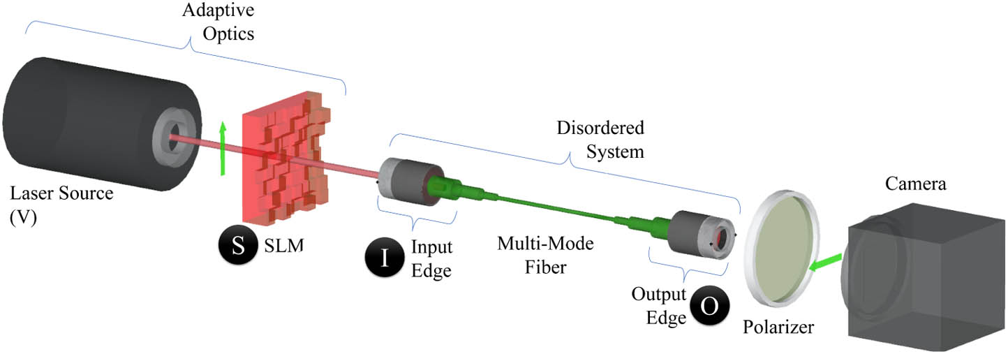
    Fig. 1. Scheme of the setup used for our imaging experiments. A laser source (vertical polarization) is modulated into a probing pattern using a spatial light modulator (SLM). Once modulated, the field is projected onto the input edge of a multi-mode fiber (I). The light that trespasses the disordered medium is imaged at the output edge (O) by a standard camera sensor (horizontal polarization).
    Scheme of the Gerchberg–Saxton phase retrieval protocols used in our manuscript. The orange box indicates where the smoothing operation takes place. Without this operation, the phase retrieval protocol is the same as described in Ref. [16].
    Fig. 2. Scheme of the Gerchberg–Saxton phase retrieval protocols used in our manuscript. The orange box indicates where the smoothing operation takes place. Without this operation, the phase retrieval protocol is the same as described in Ref. [16].
    Imaging results for five input symbols obtained after a single iteration using γ=4 measurements. The first line shows the results of the standard GS, the second shows the results of GS2-1, and the third is our method. The last row is the ground truth image sent. We used a diverging color map [34] to highlight the presence of wrong negative pixel values (in red).
    Fig. 3. Imaging results for five input symbols obtained after a single iteration using γ=4 measurements. The first line shows the results of the standard GS, the second shows the results of GS2-1, and the third is our method. The last row is the ground truth image sent. We used a diverging color map [34] to highlight the presence of wrong negative pixel values (in red).
    Comparison of imaging performance of different GS algorithms. (A) Results after a single iteration, (B) after 10 iterations, (C) after 100 iterations, and (D) after 1000 iterations. The error bar represents the standard deviation of the image reconstruction over all the objects to be reconstructed.
    Fig. 4. Comparison of imaging performance of different GS algorithms. (A) Results after a single iteration, (B) after 10 iterations, (C) after 100 iterations, and (D) after 1000 iterations. The error bar represents the standard deviation of the image reconstruction over all the objects to be reconstructed.
    Comparative study on the reconstruction of images at progressively increasing sampling ratios. The block on the top shows the reconstructions after a single iteration. The bottom block shows the same study after 10 iterations. For each block, the first row shows the reconstruction results at various sampling ratios γ for the GS. The second row shows the results of GS2-1 and the third for our method. We present these results using a modified gray scale color map, where pixels turn from white to red when reconstructing negative intensities, which are not present in the original images.
    Fig. 5. Comparative study on the reconstruction of images at progressively increasing sampling ratios. The block on the top shows the reconstructions after a single iteration. The bottom block shows the same study after 10 iterations. For each block, the first row shows the reconstruction results at various sampling ratios γ for the GS. The second row shows the results of GS2-1 and the third for our method. We present these results using a modified gray scale color map, where pixels turn from white to red when reconstructing negative intensities, which are not present in the original images.
    Difference map for the NRMSE of GS and SmoothGS. Here, we considered a variable number of iterations ∈[1,20]. In the red region, our method always surpasses state-of-the-art phase retrieval methods. The color fading to white indicates that the GS method converged to the look-alike reconstruction provided with the single iteration SmoothGS.
    Fig. 6. Difference map for the NRMSE of GS and SmoothGS. Here, we considered a variable number of iterations [1,20]. In the red region, our method always surpasses state-of-the-art phase retrieval methods. The color fading to white indicates that the GS method converged to the look-alike reconstruction provided with the single iteration SmoothGS.
    Study of the reconstruction quality by changing the size of the observation window at the output. Panel (A) shows the study for γ=2.5, and (B) for γ=3.0. The situation is similar in both cases, with SmoothGS being the only protocol able to reconstruct the image. Panel (C) displays the results for γ=3.5. Here, GS21 reaches a performance similar to SmoothGS after 10 iterations. The same applies for γ=4.0 in panel (D). Reducing it, as expected, decreases the quality at any γ. However, our algorithm still outperforms current GS implementations, converging in a single iteration and providing reliable reconstructions even in the case of γ<4.
    Fig. 7. Study of the reconstruction quality by changing the size of the observation window at the output. Panel (A) shows the study for γ=2.5, and (B) for γ=3.0. The situation is similar in both cases, with SmoothGS being the only protocol able to reconstruct the image. Panel (C) displays the results for γ=3.5. Here, GS21 reaches a performance similar to SmoothGS after 10 iterations. The same applies for γ=4.0 in panel (D). Reducing it, as expected, decreases the quality at any γ. However, our algorithm still outperforms current GS implementations, converging in a single iteration and providing reliable reconstructions even in the case of γ<4.
    Reconstruction quality as a function of resized output. Panel (A) γ=2.5 and (B) γ=3.0 report similar situations: SmoothGS is the only protocol capable of reconstructing the image in this regime. In panel (C) γ=3.5, and in panel (D) γ=4.0; GS21 reaches similar reconstructions as in SmoothGS after 10 iterations and does not converge in a single iteration. We notice how decreasing the magnification of the output observation preserves reconstruction quality up to around 0.4×. Down to this value, SmoothGS preserves its advantage over standard GS implementations even when no local correlations are expected.
    Fig. 8. Reconstruction quality as a function of resized output. Panel (A) γ=2.5 and (B) γ=3.0 report similar situations: SmoothGS is the only protocol capable of reconstructing the image in this regime. In panel (C) γ=3.5, and in panel (D) γ=4.0; GS21 reaches similar reconstructions as in SmoothGS after 10 iterations and does not converge in a single iteration. We notice how decreasing the magnification of the output observation preserves reconstruction quality up to around 0.4×. Down to this value, SmoothGS preserves its advantage over standard GS implementations even when no local correlations are expected.
    Temporal performance of the Gerchberg–Saxton phase retrievals. In panel (A), the average time per iteration is measured by running 103 cycles of the different GS implementations. In panel (B), we report the computational single-iteration time variation in percent against the GS implementation. If we call tGS the reference time, the percent variation is calculated as (tmethod−tGS)/tGS. We notice how carrying out the smoothing step at the transmission matrix permits us to keep the speed similar to that of standard GS approaches. We discuss this in Appendix E.
    Fig. 9. Temporal performance of the Gerchberg–Saxton phase retrievals. In panel (A), the average time per iteration is measured by running 103 cycles of the different GS implementations. In panel (B), we report the computational single-iteration time variation in percent against the GS implementation. If we call tGS the reference time, the percent variation is calculated as (tmethodtGS)/tGS. We notice how carrying out the smoothing step at the transmission matrix permits us to keep the speed similar to that of standard GS approaches. We discuss this in Appendix E.
    Daniele Ancora, Lorenzo Dominici, Antonio Gianfrate, Paolo Cazzato, Milena De Giorgi, Dario Ballarini, Daniele Sanvitto, Luca Leuzzi. Speckle spatial correlations aiding optical transmission matrix retrieval: the smoothed Gerchberg–Saxton single-iteration algorithm[J]. Photonics Research, 2022, 10(10): 2349
    Download Citation