One of the great efforts in modern optics is the exploitation of disordered structures for imaging and focusing through (or, perhaps, inside) optical materials. The revolution started by using light shaping devices to manipulate the light field, observing how the turbid medium reacts to controlled excitations [1]. Initially, imaging procedures were accomplished mainly by taking advantage of the memory effect [2], whereas, for focusing, feedback-based genetic algorithms were common [3,4]. However, the light propagation through a scattering device can be modeled as a linear process, in which a complex and unknown transmission matrix (TM) deterministically controls how the light is transported by the medium [5,6]. Rapidly, measuring the TM became a successful approach for turning turbid devices into standard optical tools, stimulating intense research activities [7]. Because of this, researchers developed many approaches for the recovery of TM in different scenarios (see Ref. [8] and references therein). Among these, holography requires accessing both edges via an interferometric configuration [9]. Although complex to implement, these setups provided thriving results. For holographic imaging, the usage of the reference arm permitted obtaining complete control over the image transmission through disordered channels [10]. Recently, compressed sensing approaches were used to recover the optical TM of multi-mode (MM) fiber with a reduced number of probing measurements [11]. Information about coherence within spatial and angular windows (the memory effect) was also exploited to assist the recovery of the TM in an MM fiber [12].

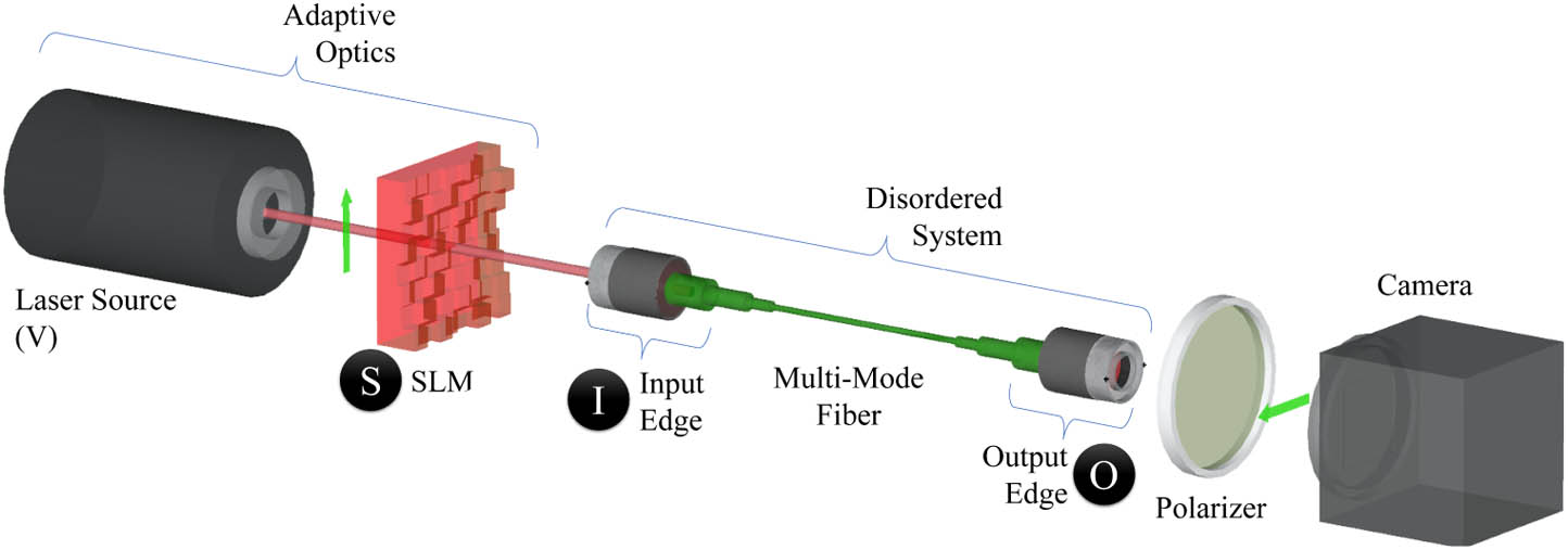
Although the holographic approach allows accurate characterization of the transmission, it is of difficult applicability in the real-measurement scenario. The presence of the reference arm, external to the fiber bundle, hinders the miniaturization of the optical device. This fact stimulates the investigation in non-interferometric configurations [13,14]. As schematized in Fig. 1, a straightforward imaging setup consists of using a light shaping device to send a given pattern on the input side of a disordered medium (an MM fiber, in our case) and recording its transmission at the output edge with a camera. Initially, the transmission recovery in such a simple configuration was done by keeping a portion of the spatial light modulator (SLM) fixed, using it as a self-reference for the characterization [6,15]. Successively, using random measurements also provided excellent frameworks for the TM reconstructions with the reference-less prVBEM Bayesian approach [14], or with Gerchberg–Saxton iterative approaches [16]. Furthermore, measurements done on the Hadamard basis have permitted the approximation of the TM using only real-valued entries [17]. These methods are supervised inversions, meaning that a known sequence of patterns is sent, and the related output fields are measured. Repeating this procedure several times, one can gain complete knowledge of the scattering process that the light field undergoes during propagation. Usually, the higher the number of patterns sampled, the better the estimation of the matrix is.

Once recovered, the TM can be used to produce a focus on a user-specified position or to invert the scattering process, directly recovering images on one edge. In both applications, the statistics of the speckle pattern produced by the light transmission through the random medium tells us information about its optical response [18]. A fundamental property is that a point source produces a speckle whose auto-correlation sets the optimal resolution achievable by the system [19,20]. This quantity is connected to the point spread function (PSF) in the propagation through homogeneous media. When analyzing a speckled image, there are regions of coherence that are, in general, larger than a single pixel. The vast majority of these methods to reconstruct the TM assume a “single-pixel camera” approach, which delineates a separable problem at the output plane. That implies that each calibration pattern sent at the input contributes independently to the output of every single pixel. Such a simplistic assumption uses less memory and is very useful for algorithm parallelization, but it discards neighboring interactions that are potentially useful. Different approaches have tried incorporating information encoded in spatial correlations, particularly those dictated by the memory effect [11,12,21]. In this study, we decided to exploit the physical information provided by the speckle statistics to aid the reconstruction of the TM. We implement our strategy by proposing a modified, non-interferometric, Gerchberg–Saxton (GS) phase retrieval (PR) approach for imaging through disorder. GS implementations have, in fact, the advantage of being the fastest framework for reconstructing the TM [22]. In a nutshell, our modification consists of linking adjacent pixels in the output plane by adding a step of image convolution with a tunable kernel. The idea takes inspiration from the oversampling smoothness (OSS) protocol, which is an algorithm proposed to suppress noise outside the support region in a Fourier PR set for imaging [22]. Here, contrarily to OSS, the smoothing step is used to couple adjacent output pixels according to the physical connection described by the average speckle size. To test the effectiveness of our modification, we decided to tackle the problem of imaging through MM fiber, performing a complete study on the number of patterns and iterations needed to achieve optimal reconstruction results. Compared to state-of-the-art methods, our algorithm converges within a single iteration and can reconstruct images using undersampled measurements. We begin our study by describing the protocol and the non-interferometric experimental setup used for imaging. After this, we will present a numerical study based on the experimental measurements to characterize the behavior of our method, discussing the results and additional perspectives.

As described by Goodman [23], the speckles distributed in a pattern produced by a scattering medium have an average size that can be estimated via its auto-correlation. For fully developed speckles, the auto-correlation turns out to be a sharply peaked function since the average speckle size is of the order of the wavelength. Such dimension is typically much smaller than currently available camera pixels; thus, the auto-correlation in this regime reduces to that of a broadband noise [24]. If we call S the speckle pattern recorded by the camera, this implies that the auto-correlation in the discretized imaging plane is S⋆S≈δ, where δ is the Dirac distribution and ⋆ is the cross correlation operator. Within the memory effect range approach [2,24], this property was exploited to perform hidden imaging based on direct speckle observation. Experimentally, however, we are far away from obtaining a delta function. The fact that the auto-correlation is not point-like implies that neighboring modes detected by the camera are not independent completely but, instead, are spatially correlated on the plane. For the purpose of our study, we can assume that the speckles exhibit a Gaussian auto-correlation, S⋆S=g(Σ), of which its extent can be approximated by recovering its standard deviation Σ. In the following, we exploit this information to allow our method to converge faster than state-of-the-art implementations. So far, many TM recovery approaches proposed consider each pixel in the output edge independent of each other. Here, instead, we include neighboring interaction by introducing a step in the GS algorithm that couples the output pixels via the system’s expected PSF, providing imaging benefits in terms of reconstruction efficiency.

PR is a class of algorithms aiming at the recovery of the phase of a wavefront given a set of intensity measurements. The problem we analyze can be formalized as a linear field combination, which results in the formation of a disordered speckle pattern on the output edge of the MM fiber. By using the camera pixels as a spatial unit for length, we describe the problem as follows. We send a set of random binary patterns of size Ni=L×L from the input edge modulated by the SLM. Even if the patterns are bi-dimensional, we store them as single dimension arrays within the probing matrix P, so each row in P represents a given pattern. In general, we consider a variable number of measurements M (each corresponding to a different input pattern) so that P has a dimension of M×Ni. We assume that the disordered medium can be described by an unknown complex TM X, which scrambles the input P into the output measurements Y, with each measurement composed by No output pixels. The underlined linear transmission model can be written as Y=PXT.(1)

The matrix XT has a size of Ni×No, and the output matrix Y has dimensions of M×No. The goal of the PR problem is to find X, given the probing matrix P and the sole measurement of the modulus |Y|. In our case, in fact, the camera records the field intensity I=|Y|2, which stores every speckle pattern S obtained in response to each input pattern. We refer to it as PR because the method retrieves the phase of the output Y and, consequently, lets us estimate X. As already mentioned, the class of PR problems was tackled in several ways, such as with the EKF-MSSM approach [25], SDP algorithm [26,27], prVBEM [14,28,29], GAMP [30] and its extension GVAMP [31]. However, these algorithms are computationally demanding, whereas GS approaches represent the fastest and workflow efficient alternatives, as thoroughly discussed by Huang et al. [16]. The GS PR is, in fact, a simple and efficient protocol based on an iterative approach, which we schematically describe in Fig. 2. The method begins by assigning a random phase Φ0 to the measured intensity to form the (complex) estimated output observation, Y0=AeΦ0. Here, A=I is the squared root of the intensity detected on the camera. Since the method is based on forward and backward application of the measurement patterns, we pre-compute the Moore–Penrose pseudo-inverse [32] of the matrix P, which we denote with P†.

The method that we propose consists of five steps schematized in Fig. 2. 1.First, we form an estimation of the complex output field Yi keeping the recorded modulus A and associating a phase from the previous iteration. In the beginning, the phase Φ0 is initialized by extracting random numbers from a uniform distribution.2.We use the output estimation to compute the new guess for the TM as Xi=P†Yi.3.We let the sequence of input patterns P propagate through the retrieved TM, and we calculate the new output estimation as Y˜i=PXiT.4.We convolve the predicted output Y˜i with a smoothing Gaussian kernel, setting its variance as a function of the iteration number.5.We keep the phase of the estimated output as Φ˜i+1=Arg{Y˜i+1}, and we pass it to step 1, restarting the cycle.

We refer to our method as SmoothGS (where appropriate, also abbreviated with SGS). When the smoothing kernel tends to a δ-function, the iteration described reduces to the standard GS PR [16]. As a rule of thumb, we decided to vary the neighboring interaction size by controlling the sigma of the Gaussian kernel. The first iteration starts with half the standard deviation determined by the fit of the auto-correlation with a Gaussian function, σ=Σ/2 (see Appendix D). Such kernel g(σ) represents a Gaussian ensemble average of the speckle size observed in the fiber. The value is decreased linearly as a function of the number of steps to σ=0.1 pixels, which returns approximately a delta function. In a discretized kernel, the latter corresponds to an image with only the central pixel having a non-null value, whereas all the surrounding is set to zero. In this way, we allow for a strong neighboring coupling at the beginning of the iteration and weaken its effect as the iteration proceeds. After a certain number of iteration steps, we recover the TM that describes the system.

On the other hand, the imaging procedure consists of sending an unknown pattern to the input edge and reconstructing it based on the speckle recorded at the output and the estimated TM. The problem to be solved, in this case, is analogous to the previous one: (Y′)T=X(P′)T,(2)where (Y′) is the set of the observed speckle patterns and (P′) represents the unknown images on the input edge that generated it. For our study, we use a double PR approach [14,33]. The first PR is in charge of retrieving the TM; the second carries out the image reconstruction. Since Huang et al. [16] have already studied the recovery performance of GS methods, we decided to complement their work by using a double PR approach to assess the correct recovery of the transmission. Since the second retrieval stage is strongly influenced by the first, we study whether the protocol can recover images from the input edge, monitoring the diagonality of the focusing operator calculated using the recovered TM.

In our study, we are interested in the characterization of a disordered device in a non-interferometric setup, which we sketched in Fig. 1. A single-mode continuous-wave He–Ne laser source (wavelength λ=632.8nm, vertically polarized) is coupled to an SLM (pixel size 20 μm), which controls the field that enters the disordered device. The beam is expanded 10× with a two-lens telescope, covering a circular portion of the SLM with a radius of 0.4 cm. The light modulated by the SLM is demagnified 7.5× with a two-lens telescope and injected into the input facet (I) of an MM fiber (1.08 m long step-index fiber, 1 mm core diameter, numerical aperture NA=0.39, refractive indices ncore=1.457, ncladd=1.404) and undergoes random scattering events during its propagation. We record the propagated intensity field on the output facet (O) with a 3× magnification objective, selecting the horizontal polarization. The polarized detection guarantees that the transmission problem is scalar, and, in the case of interest, one may want to repeat the procedure for the vertical polarization also. We decided to divide the illuminated SLM area impinging on the input edge into 24×24 segments, consisting of 11×11 SLM pixels each, and we analyze a squared window of 256×256 pixels within the central core of the output edge of the MM fiber. The region we use is delimited with a square box on the speckle pattern of Fig. 2. Since we control N=576 segments of the SLM, it is convenient to define the sampling ratio as γ=M/N, and we are interested in evaluating how the algorithm behaves as a function of γ. Then, we send a total of Mtot=10N patterns for the characterization, and, consequently, we record the same number of speckle realizations S. In this representation, γ=1 means that the number of measurements matches the number of pixels controlled at the SLM. These measurements, then, are used to characterize the TM. Instead, for the imaging procedure, we send 400 letters randomly extracted from the Greek alphabet. These images are structurally different from the random images used for training and not used during the characterization. We show a few examples in the bottom row of Fig. 3; these are the objects we aim at reconstructing.

After acquiring the experimental measurements, we employ the double PR method: the first is to reconstruct the TM of a generic MM fiber, and the second is to recover the unknown symbols transmitted through it. Here, we discuss the results obtained with our protocol against the reconstructions provided by standard PRs described in the literature. The results presented are experimental entirely, and we organize our study as follows. To retrieve the TM, we make use of binary random patterns only, and we run independent PRs using different sampling ratios, γ, ranging from 0.5 to 10, increased in steps of 0.5. Although not explicitly reported, the convergence of the TM was monitored by looking at the unitarity of the focusing operator, X†X. For the imaging procedure, we use only the speckle patterns obtained by the propagation of the Greek letters through the MM fiber. These symbols are used for the assessment of the reconstruction quality as a function of the number of iterations performed. The metric chosen to compare the reconstructed images with the ground truth is the normalized root-mean-square error (NRMSE). By definition NRMSE ranges from 0 to 1, and a lower value corresponds to a better reconstruction. If we call p′(x,y) the reconstructed image and p(x,y) the original object transmitted, we have the following: NRMSE=1−max|p′(x,y)⋆p(x,y)|2∑x,y|p′(x,y)|2∑x,y|p(x,y)|2.(3)

We begin our study by running independent double PRs used for reconstructing the test images, varying the number of calibration patterns in combination with a variable number of iterations. For comparison, we make use of the standard GS and improved GS2-1, proposed by Ref. [16], that we use as the reference against our method. In Fig. 3, we report the image reconstructions of a few symbols recovered after a single iteration of the three GS methods. In this case, a single iteration implies a single GS-step for both the TM reconstruction and the imaging procedure, with a sampling ratio of γ=4. The two state-of-the-art GS methods return solutions that are not yet formed, with poor contrast and a noisy background (Fig. 3, rows 1 and 2). Our method (Fig. 3, third row), instead, immediately achieves results much closer to the ground truth solution (Fig. 3, fourth row). To enrich our analysis, we performed a study by varying the number of the iterations over 3 orders of magnitude: 1, 10, 100, and 1000 steps. In Fig. 4, we plot the different NRMSE obtained at the end of each reconstruction run. The error bars are obtained from the reconstruction statistics over all the symbols considered in each experiment. First, we noticed that it is impossible to achieve any good result for γ<1, as further confirmed by the fact that the focusing operator does not exhibit diagonality in any of the methods used. This impossibility is due to the fact that, at this sampling ratio, the P is hard to invert. For γ=1, instead, the optimal result is readily provided by all the methods. Reconstructions at this regime exhibits a constant behavior for any number of iterations. We point out that, only in this particular case, the sampling matrix P is squared, and so, the inverse is well-defined as P†=P−1. Ideally, by increasing the samples used for the reconstruction, one would expect the results to get progressively better. Instead, the GS and GS2-1 exhibit a performance drop that does not improve by running longer iterations for any γ∈(1,4). In this regime, we note that GS2-1 performs better than standard GS, as also reported by Huang et al. [16], but none of them reconstruct a diagonal focusing operator. This fact implies that, in this sampling regime, the matrix recovered by GS and GS2-1 cannot provide focusing or imaging capabilities. For γ≥4 and after 10 iterations, the reconstruction quality improves (and the focusing operator becomes diagonal), though it progressively deteriorates when increasing the number of iterations. This behavior makes selecting the correct iteration number crucial for the GS and GS2-1 methods.

With our method, instead, we obtain stable performances regardless of the number of iterations. For any γ in Fig. 4(A), it appears evident that the smoothed implementation of the GS achieves the optimal imaging performance after just a single iteration cycle. The result is maintained up to thousands of iterations, showing excellent numerical stability. Remarkably, our method always outperforms the state-of-the-art in the downsampled regime γ∈(1,4) (the four-phase method [6,35] and the three-phase method [36]). The same conclusions apply to the focusing operator, which constantly resulted in a diagonal shape and improved when we increased the sampling ratio, enabling light delivery control even in undersampled scenarios. To ease the analysis, we report the direct imaging performance after 1 (top group) and 10 (bottom group) iterations in Fig. 5. After a single iteration, SmoothGS turns out to be always better than the other GSs, progressively increasing the reconstruction quality for higher sampling ratios. After 10 iterations, the other methods approach the same imaging quality obtained by our implementation, exhibiting a visible discontinuity at γ=3.5.

From the previous analysis of the plots in Fig. 5, we notice that our method is robust and does not deteriorate when exceeding the iteration number. Furthermore, reconstructions continuously improve as more data are used in training, i.e., as γ increases. Indeed, not only the SmoothGS performs better than recent GS-based algorithms at every γ value, but it also displays no efficiency barrier in γ. Up to the state-of-the-art, we can consider this to be the optimal result achievable in imaging with GS-based solutions. Thus, we use our method as a reference, and we compare the imaging NRMSE obtained with GS2-1 by solving image reconstructions over 1 to 20 iterations. The difference map between SmoothGS and GS2-1 is reported in Fig. 6: the whiter the region, the closer the results are between the two methods. After a single iteration, our method is unbeaten for any sampling ratio considered. After two iterations, both methods provide identical results only if γ>7; after three iterations, the sampling ratio can decrease to γ>5 with GS2-1. However, this trend rapidly saturates, and, for γ∈(1,3), no solutions provided by the current methods can approach the image quality provided by ours.

To further assess the validity of our reconstruction protocol, we perform another study as a function of the output size used for the transmission recovery. We begin by reconstructing the TM when reducing the number of pixels in the cropped window. The performance obtained at different γ is reported in Fig. 7. As expected, reducing the number of observed modes in the output has a negative effect on the overall reconstruction quality. Our method, however, still provides the best solution after a single iteration, even at γ<4, where standard GS2-1 fails or needs more iterations to converge. It is important to recall that we are not changing the average speckle size when reducing the cropping window. To understand what happens when we reduce the speckle size, we perform a similar study by demagnifying the output observation. In this case, we assume the smoothing rule is unchanged with σ=2 pixels (Fig. 8). In principle, keeping the same smoothing is a wrong assumption because resizing the pattern reduces the average speckle size, and we should reduce σ accordingly. In particular, magnifying with a factor of 0.5 destroys the average correlation length in the speckles, which now appears as wide as a single pixel. Remarkably, our method still provides the best reconstructions after a single iteration, even when local correlations are no longer expected. We notice that the reconstruction performances remain unchanged down to 0.5, after which they start to degrade remaining, however, always better than GS2-1. The physical meaning of the smoothing operation is lost in this case, but the blurring operation still operates as a regularization term for the inverse problem solution.

In our article, we described how the introduction of a convolution step in a PR GS implementation considerably improves reconstruction results. Although a single iteration of our algorithm takes a little longer than the single iteration in state-of-the-art PR algorithms, in SmoothGS, one is enough to get straight to the optimal reconstruction. A single cycle of SmoothGS consists of five operations, whereas the GS and GS2-1 discussed above consist of four. To compare the computational cost, we decided to test the average computing time of the three methods. We averaged 103 iterations comprising the memory transfer between the CPU and GPU memory. We report the average seconds per step in Fig. 9(A) and the time variation against the simplest GS in the plot below. As expected, GS and GS2-1 almost require the same time to carry out a single iteration, with the second being only 3% slower. Our method, instead, is 50% slower on a single cycle when smoothing the output. This increased computational cost is uniquely attributable to the convolution step, which needs to be done at each of the M=γN recorded outputs. A clever choice, instead (as discussed in Appendix E), is to apply the smoothing rule directly to the TM because, contrarily to the output Y, its dimension does not change with γ. In both cases, the results are identical, but the row-column multiplications to be carried out are less when γ>1. This trick permits us to keep the performance very close to that of standard GS, in particular when increasing the sampling ratio. Even in the worse case, however, a single SmoothGS iteration is still less expensive than performing two GS iterations (and it could take tens of those to converge to an effective reconstruction; see Fig. 5). This empirical property guarantees that our method is always faster in converging than any competitor. SmoothGS readily provides the best reconstruction achievable with the minimum temporal requirement. As a final remark, in our current implementation, the acquisition speed reaches 4.5 frames per second, which implies that to sample at γ=2, the measurement lasts 256 s. Even if we are close to the actual limit of our hardware, which is 5.5 frames per second, the main responsibility for this is the SLM that needs 170 ms to refresh. This bottleneck makes the measuring time much greater than the length of time that SmoothGS takes to reconstruct the TM (less than 0.1 s, on average and excluding camera/memory data transfer). On the other hand, this implies that we could update a new estimation of the TM in between two successive measurements, giving room to follow the TM evolution in time. However, we designed this study in such a way that it prescinds the actual hardware used. Using a faster camera and a digital micromirror device (DMD) in place of the SLM could dramatically decrease the measuring time, leaving the setup design practically unchanged. However, this depends on the technology level that is currently available, not on the overall methodology employed. The same applies, of course, to computational hardware. The next generation of GPUs will most likely beat current performance in terms of pure computational time [Fig. 9(A)] but will most probably have the same relative gain [Fig. 9(B)]. In this spirit, we feel that a discussion about these absolute numbers will not add much in terms of scientific content, and we leave this discussion to a more technical study.

At high γ, the fact that our algorithm converges in one cycle to the same result provided by GS and GS2-1 can be qualitatively extrapolated by looking at the reconstructions in Fig. 5. The bottom row clearly shows that all the methods reconstruct the Λ object with a peculiar artifact (the black dot on the upper right corner). In this sampling regime, it is not the reconstruction that improves but rather the way we reach it. Converging in one cycle eliminates the burden of determining the number of iterations, which, in inverse problems, is a parameter of the algorithm that needs to be determined. On the other hand, the fact that a solution can also be achieved in the low sampling regime γ=(1,4) is a clear sign of a phase transition in the algorithm (Fig. 4). Additionally, we remark that the transition strongly depends on the iteration number in GS and GS2-1, whereas SmoothGS does not show appreciable differences. The regularization seems to have a decisive impact more on the algorithm behavior than on its capability of finding different solutions. We believe that further investigations are worthwhile to study this regularizing effect.

By smoothing the output of the GS, we introduced a model-based regularizer controlled by the statistics of the speckles [23]. Our idea comes when noticing that current methods in TM reconstruction typically neglect neighboring interactions. The independence of the output pixels permits the separation of the problem, so it requires less memory, and the computational workflow is easy to distribute. However, high memory GPU solutions currently provide enough computational power to carry out the whole task in a single graphic card. Since our method computes neighboring interactions at the output plane, the whole dataset needs simultaneous processing. Fitting everything in a single GPU avoids the bottleneck of CPU-GPU memory transfer that would render our method unfeasible in terms of computation time. In particular, the constant development of convolutional neural network strategies makes it easy to design numerical algorithms that implement depth-wise convolutions in image processing [37] with PyTorch [38]. This constant increase in computational performance is beneficial to our implementation, permitting us to process images with a high number of pixels.

Since TM can be used to engineer the focusing capability of the system [39], we can ease its reconstruction when strong non-local correlations are present. A relevant case is with amorphous speckles [40], which exhibit quasi-Bessel focusing [20] that implies non-Gaussian kernels. In these cases, however, a Gaussian fit is not a good choice anymore to recover the smoothing kernel: one may need to invert the speckle auto-correlation to find a good kernel candidate. Last but not least, the ability to obtain meaningful reconstructions at a low sampling ratio, γ<4, is an interesting feature provided by our method. The four-phase [6,35] and the three-phase methods [36] set the minimum number of measurements as 4N and 3N, respectively, relying on dephased versions of the same input patterns. Our method is more general, accepts random sampling, and could work even with less than 3N measurements. Furthermore, SmoothGS has proven robustness against the wrong choice of iteration number and always converged within one cycle. Lastly, it exhibited a predictable behavior as a function of the sampling ratio with a little computational burden compared to standard GS implementations. These characteristics are crucial aspects for the scientific community that aims to reduce the number of acquisitions, and we strongly believe that it is worth investigating further. For example, considering the information about the polarization of the observed output field could improve the reconstruction further [41], in particular, when aiming at the temporal characterization of the fiber. In fact, it is well known that the TM changes by bending the fiber or varying its temperature [42]. In this context, the ability to constantly correct the TM comes in hand with the possibility of reconstruction using the fewest number of measurements possible. In this context, a stochastic choice of the training patterns may help GS algorithms to converge faster [43]. The assumption on sparsity in the TM [11] and iterative focusing via binary phase-only patterns [44] have already shown a promising reduction in the number of measurements needed. The development of fast TM reconstruction frameworks is, indeed, of fundamental interest in biomedical imaging, and PR algorithms are promising resources [45]. There is an increasing interest in endoscopy using MM fibers. In our case, after initial characterization, the role of the input/output edges is reversed for imaging, as in Ref. [15]. This configuration implies that the edge used to send the light in now has to be used to gather the light from the sample we want to image. With this work, then, we try to pave the road toward new computational methods that are fast and measurement efficient. In our current implementation, SmoothGS can recover the TM in 0.1 s (at γ=2), giving room for developing new strategies for following its evolution over time. In this respect, our contribution may assist the definition of clinical tools for non-invasive and real-time optical measurement.

Acknowledgment. We acknowledge the support from the ERC under the European Union’s Horizon 2020 Research and Innovation Program, Project LoTGlasSy, and Prof. Giorgio Parisi. We also acknowledge the support of LazioInnova - Regione Lazio under the program Gruppi di ricerca 2020 - POR FESR Lazio 2014-2020, Project NanoProbe. Author contributions: D. A. and L. L. conceived the idea and wrote the manuscript. D. A. designed the code and performed numerical studies. L. D., A. G., P. C., M. D. G., and D. B. set up the experimental acquisition. D. S. coordinated the experiments. L. L. supervised the project. All the authors reviewed the manuscript.