• Photonics Research
  • Vol. 11, Issue 1, 27 (2023)
Minru He1、2, Yansheng Liang1、2、4、*, Xue Yun1、2, Zhaojun Wang1、2, Tianyu Zhao1、2, Shaowei Wang1、2, Piero R. Bianco3, and Ming Lei1、2、5、*
Author Affiliations
  • 1MOE Key Laboratory for Non-Equilibrium Synthesis and Modulation of Condensed Matter, School of Physics, Xi’an Jiaotong University, Xi’an 710049, China
  • 2Shaanxi Province Key Laboratory of Quantum Information and Quantum Optoelectronic Devices, School of Physics, Xi’an Jiaotong University, Xi’an 710049, China
  • 3Department of Pharmaceutical Sciences, College of Pharmacy, University of Nebraska Medical Center, Omaha, Nebraska 68198-6025, USA
  • 4e-mail: yansheng.liang@mail.xjtu.edu.cn
  • 5e-mail: ming.lei@mail.xjtu.edu.cn
  • show less
    DOI: 10.1364/PRJ.474065 Cite this Article Set citation alerts
    Minru He, Yansheng Liang, Xue Yun, Zhaojun Wang, Tianyu Zhao, Shaowei Wang, Piero R. Bianco, Ming Lei. Generalized perfect optical vortices with free lens modulation[J]. Photonics Research, 2023, 11(1): 27 Copy Citation Text show less
    Principle of the FLM method. (a) Abridged general view of the free lens modulation (FLM) method. (b) Superposition of the annular lens and the vortex phase to generate the free lens. (c) Models of various free lenses and the corresponding GPOV profiles.
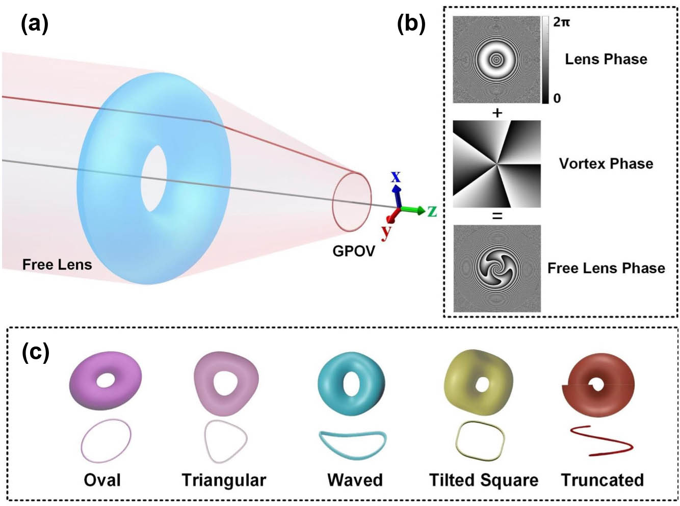
    Fig. 1. Principle of the FLM method. (a) Abridged general view of the free lens modulation (FLM) method. (b) Superposition of the annular lens and the vortex phase to generate the free lens. (c) Models of various free lenses and the corresponding GPOV profiles.
    Experimental layout. (a) Light path diagram. (b) Experimental setup. ① Laser with λ=1064 nm, ② SLM, ③ objective lens, and ④ CMOS camera.
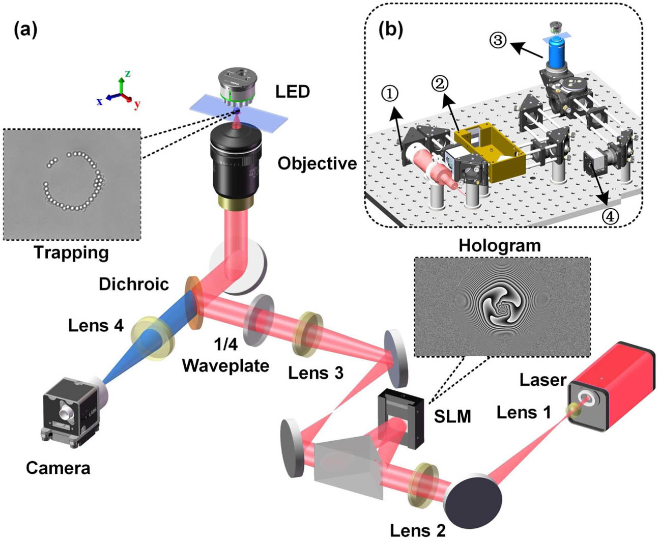
    Fig. 2. Experimental layout. (a) Light path diagram. (b) Experimental setup. ① Laser with λ=1064  nm, ② SLM, ③ objective lens, and ④ CMOS camera.
    Generation of annular POVs. (a) Simulated intensity distribution and (b) simulated phase distribution of the annular POVs with TCs l=1 and 80. Scale bar: 1 mm. (c) Radius plot of annular POVs, with TCs l=1−80. (d) Experimental intensity distribution and (e) measured interference patterns of the annular POVs with TCs l=1 and 80. Scale bar: 20 μm. (f) Radius plot of annular POVs, with TCs l=1−80.
    Fig. 3. Generation of annular POVs. (a) Simulated intensity distribution and (b) simulated phase distribution of the annular POVs with TCs l=1 and 80. Scale bar: 1 mm. (c) Radius plot of annular POVs, with TCs l=180. (d) Experimental intensity distribution and (e) measured interference patterns of the annular POVs with TCs l=1 and 80. Scale bar: 20 μm. (f) Radius plot of annular POVs, with TCs l=180.
    Generation of 2D GPOVs. (a) Free lens models. (b) Simulated light field models. (c) The phase of the free lenses in (a) with TC l=1. (d), (e) Experimentally generated light fields for l=1 and 80 using the oval, triangular, square, and pentagonal free lenses, respectively. Scale bar: 20 μm.
    Fig. 4. Generation of 2D GPOVs. (a) Free lens models. (b) Simulated light field models. (c) The phase of the free lenses in (a) with TC l=1. (d), (e) Experimentally generated light fields for l=1 and 80 using the oval, triangular, square, and pentagonal free lenses, respectively. Scale bar: 20 μm.
    Generation of 2D GPOVs with different parameters. (a) Model of different free lenses. Variation of the smoothness of the light fields with parameter of (b) p=5, (c) p=10, (d) p=15, and (e) p=20 for GPOVs. Scale bar: 20 μm.
    Fig. 5. Generation of 2D GPOVs with different parameters. (a) Model of different free lenses. Variation of the smoothness of the light fields with parameter of (b) p=5, (c) p=10, (d) p=15, and (e) p=20 for GPOVs. Scale bar: 20 μm.
    Generation of 3D GPOVs (see Visualization 1). (a) Free lens models of different 3D GPOVs, including the tilted annular, waved annular, tri-waved annular, truncated annular, tilted oval, tilted triangular, tilted square, and tilted pentagonal, respectively. (b) Simulated light field models corresponding to (a). (c) Calculated free lens phase. (d) Side view of the rendered 3D light fields (scale bar: 20 μm) of different 3D-GPOVs. (e)–(g) Measured light intensity distribution in the x-y plane at different z positions, Scale bar: 20 μm. First line: the 1D intensity profile of Position 1, Position 2, and Position 3. (h) Normalized intensity, (i) transverse FWHM, and (j) axial FWHM of tilted annular 3D GPOVs (see Visualization 2) with increasing tilt angle in different 3D positions corresponding to Position 1, Position 2, and Position 3.
    Fig. 6. Generation of 3D GPOVs (see Visualization 1). (a) Free lens models of different 3D GPOVs, including the tilted annular, waved annular, tri-waved annular, truncated annular, tilted oval, tilted triangular, tilted square, and tilted pentagonal, respectively. (b) Simulated light field models corresponding to (a). (c) Calculated free lens phase. (d) Side view of the rendered 3D light fields (scale bar: 20 μm) of different 3D-GPOVs. (e)–(g) Measured light intensity distribution in the x-y plane at different z positions, Scale bar: 20 μm. First line: the 1D intensity profile of Position 1, Position 2, and Position 3. (h) Normalized intensity, (i) transverse FWHM, and (j) axial FWHM of tilted annular 3D GPOVs (see Visualization 2) with increasing tilt angle in different 3D positions corresponding to Position 1, Position 2, and Position 3.
    Capture performance of annular POVs (see Visualization 3). (a) Screenshot of the rotated particle in an annular POV. Scale bar: 10 μm. Particle size: 3 μm. (b) Time-lapse image of the captured particle in an annular POV. (c) Rotation rate against the TC.
    Fig. 7. Capture performance of annular POVs (see Visualization 3). (a) Screenshot of the rotated particle in an annular POV. Scale bar: 10 μm. Particle size: 3 μm. (b) Time-lapse image of the captured particle in an annular POV. (c) Rotation rate against the TC.
    Capture performance of GPOVs (see Visualization 4). Screenshot and time-lapse of captured particles by the (a) oval GPOV, (b) triangular GPOV, (c) square GPOV, and (d) pentagonal GPOV with TC l=20. Scale bar: 10 μm; particle size: 3 μm.
    Fig. 8. Capture performance of GPOVs (see Visualization 4). Screenshot and time-lapse of captured particles by the (a) oval GPOV, (b) triangular GPOV, (c) square GPOV, and (d) pentagonal GPOV with TC l=20. Scale bar: 10 μm; particle size: 3 μm.
    Minru He, Yansheng Liang, Xue Yun, Zhaojun Wang, Tianyu Zhao, Shaowei Wang, Piero R. Bianco, Ming Lei. Generalized perfect optical vortices with free lens modulation[J]. Photonics Research, 2023, 11(1): 27
    Download Citation