Generalized perfect optical vortices with free lens modulation

Minru He; Yansheng Liang; Xue Yun; Zhaojun Wang; Tianyu Zhao; Shaowei Wang; Piero R. Bianco; Ming Lei

doi:10.1364/PRJ.474065

Abstract

In this paper, we present an approach called the free lens modulation (FLM) method to generate high-perfection 3D generalized perfect optical vortices (GPOVs) with topological charges of 1–80. In addition, 2D and 3D GPOVs were produced by altering the parameters of the freely shaped lenses. To verify the quality of the GPOVs produced with the FLM method, we conducted optical trapping experiments and realized linear control of the rotation rate of the trapped particle. Due to the great advantages of high perfection and high power usage in generating arbitrarily shaped GPOVs, the FLM method is expected to be applied in optical manipulation, optical communications, and other fields.

1. INTRODUCTION

Optical vortices (OVs) [1] are optical beams with helical wavefronts, i.e., a phase term of $\exp (i l φ)$ with $l$ denoting the topological charge (TC). This helical phase distribution leads to the ring-like intensity pattern of a vortex beam and orbital angular momentum (OAM) of $l ℏ$ per photon [2]. Recently, OVs have shown a huge application potential in many fields because of their ring-like intensity patterns or the nature of OAM [3 –6]. Generally, the radii of vortex beams grow along with the increasing absolute value of the TC, which restricts the use of many applications. To break this limitation, Ostrovsky et al. [7] introduced the concept of perfect optical vortices (POVs) in 2013, which are a special type of OVs that have the radius independent of the TC and a much higher intensity gradient [8]. Theoretically, POVs are described as the Fourier transform of Bessel beams. Many efforts have been made to generate POVs [7 –17]. Most of these are based on the Fourier transform [6 –8,10 –13,18,19], or the conversion of a Laguerre-Gauss beam [9]. The unique features have also brought POVs great attention in optical manipulation [9,20 –22], optical communications [18,19], quantum optics [10], optical encryption [23], and other fields. Note that typical POVs are commonly considered to have annular intensity profiles.

Recently, arbitrarily shaped POVs, also called generalized POVs (GPOVs) [24], have been reported. GPOVs have similar properties to POVs, including a phase gradient along the narrow trajectories and independence between the intensity profile and the TC. Such light fields are no longer limited to the annular shape but show various intensity patterns, such as oval or triangular [25]. These alternately shaped POVs can provide additional possibilities in advanced applications, such as optical manipulation [26,27], single-shot lithography [28], and optomechanical assemblies [29,30]. Methods have been reported to produce GPOVs, including astigmatic transformation [31], high-order cross-phase modulation (HOCP) [32], superpixel method [24], and others [33]. Most methods are limited to generating 2D GPOVs with a small $TC (l = 1 − 16)$ , thus restricting the application of GPOVs in various areas, such as optical communications that require high information capacity or optical trapping that demands a high driving force. Rodrigo et al. [34] realized 3D polymorphic beams using complex amplitude modulation geometry. However, this approach requires simultaneous modulation of the amplitude and phase of the input beam, leading to high zero-order diffraction and low power usage, especially for a large TC.

In this paper, we present a pure-phase modulation approach called free lens modulation (FLM) to generate arbitrarily shaped, high-perfection 2D and 3D GPOVs with large TCs. The basic principle of the FLM method is to design a phase map of the shape-controllable digital lens and load it onto a pure-phase spatial light modulator (SLM). When the collimated laser passes through the SLM, a corresponding GPOV is generated at the focal region of the digital lens. Meanwhile, if we superimpose a vortex phase on the shape-controllable lens phase, arbitrarily shaped GPOVs can be generated. In this approach, a freely shaped digital lens acts like an “optical pen” to modulate and focus the laser beam. Consequently, the FLM method offers high power usage, high perfection, and high flexibility. Detailed derivation and experimental validation of the FLM method will be presented here.

Sign up for Photonics Research TOC. Get the latest issue of Photonics Research delivered right to you！Sign up now

2. METHODS

A. Principle of FLM

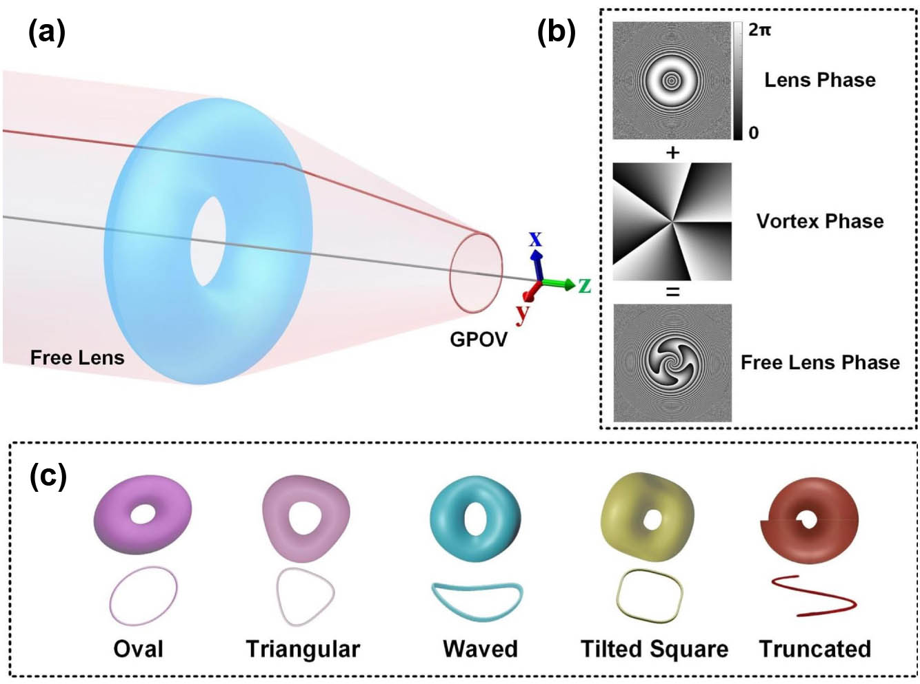
The basic idea of the FLM method is to use a freely shaped digital lens with a vortex phase to create GPOVs in the focal plane of the free lens [Fig. 1(a)]. The FLM method allows variously shaped GPOVs to be readily created, including oval, triangular, square, tilted square, and truncated ones [Fig. 1(c)]. More complex 3D GPOVs can be generated by the elaborate design of the digital lens.

Principle of the FLM method. (a) Abridged general view of the free lens modulation (FLM) method. (b) Superposition of the annular lens and the vortex phase to generate the free lens. (c) Models of various free lenses and the corresponding GPOV profiles.

Figure 1.Principle of the FLM method. (a) Abridged general view of the free lens modulation (FLM) method. (b) Superposition of the annular lens and the vortex phase to generate the free lens. (c) Models of various free lenses and the corresponding GPOV profiles.

The FLM method has high flexibility because the free lens serves as an “optical pen” in 3D. The generalized expression of the transmission function of the digital lens can be $t_{l}^{G} (r, φ) = P (r, φ) e^{- i k {(r - ρ_{0} (φ))}^{2} / 2 f (φ)} e^{i l φ},$ (1)where ( $r$ , $φ$ ) are the polar coordinates, $P (r, φ)$ represents the aperture function, $k = 2 π / λ$ refers to the illumination wavenumber, and $ρ_{0} (φ)$ and $f (φ)$ denote the shape and focal distance of the designed digital lens. The transmission function of a free lens in Eq. (1) can be considered as a superposition of the phase of a toroidal lens and a vortex lens, as shown in Fig. 1(b). Setting $P (r, φ) = 1$ and considering a uniform plane wave as the input beam, $E_{0} = A$ , with $A$ being a constant, the diffracted light field of 3D GPOVs according to Fresnel diffraction is $E (u_{0} (φ)) = A \frac{e^{i k z}}{i λ z} e^{i π ρ^{2} / λ z} F [e^{- i k {(r - ρ_{0} (φ))}^{2} / 2 f (φ)} e^{i π r^{2} / λ z} e^{i l φ}] = A \frac{e^{i k z}}{i λ z} e^{i π ρ^{2} / λ z} \iint e^{- i k {(r - ρ_{0} (φ))}^{2} / 2 f (φ)} e^{i k r^{2} / 2 z} e^{i l φ} e^{- i k ρ r \cos (θ - φ) / z} r d r d φ,$ (2)where $u_{0} (φ) = (ρ_{0} (φ), φ, f (φ))$ denotes a 3D curve parameterized by azimuthal angle $φ$ , $F [\dots]$ represents the Fourier transform, and ( $θ$ , $ρ$ ) are the polar coordinates at the Fresnel diffraction plane. Assume that the focal distance $f (φ)$ fluctuates slowly around some average value $f_{0}$ . We argue that the diffracted field will develop a 3D curve-like intensity profile of the approximate form of $u_{0} (φ)$ in the vicinity of the reference point (0, 0, $f_{0}$ ). To see this, we invoke the stationary phase method and write down the phase of the integrand in Eq. (2): $Φ (r, φ) = - \frac{k {(r - ρ_{0} (φ))}^{2}}{2 f (φ)} + k \frac{r^{2}}{2 z} + l φ - \frac{k r ρ}{z} \cos (θ - φ) .$ (3)The integral in Eq. (2) is contributed mainly by the points ( $r$ , $φ$ ) that satisfy the stationary phase conditions ${\begin{matrix} \frac{\partial Φ}{\partial r} = - k \frac{r - ρ_{0} (φ)}{f (φ)} + k \frac{r}{z} - k \frac{ρ}{z} \cos (θ - φ) = 0 \\ \frac{\partial Φ}{\partial φ} = - \frac{\partial (\frac{{(r - ρ_{0} (φ))}^{2}}{2 f (φ)})}{\partial φ} + \frac{l}{k} - \frac{r ρ}{z} \sin (θ - φ) = 0 \end{matrix} .$ (4)For a given point in the diffraction region with coordinates ( $ρ, θ, z$ ), the field there is mainly contributed by points ( $r$ , $φ$ ) on the input plane that satisfies Eq. (4).

Considering the standard planar 2D annular POV, we replace the focal length $f (φ)$ with a constant focal length $f_{0}$ and the predesigned radius $ρ_{0} (φ)$ with a constant radius $ρ_{0}$ . The POV will emerge at the diffraction distance $z$ equal to $f_{0}$ . Note that the term $\frac{{(r - ρ_{0})}^{2}}{2 f_{0}}$ is irrelevant to $φ$ ; thus, its partial differentiation of $φ$ is 0. Substituting $z = f (φ) = f_{0}$ and $ρ_{0} (φ) = ρ_{0}$ in Eq. (4), we get ${\begin{matrix} ρ_{0} - ρ \cos (θ - φ) = 0 \\ \frac{l}{k} - \frac{r ρ}{f_{0}} \sin (θ - φ) = 0 \end{matrix} .$ (5)

The solution of Eq. (5) is $ρ^{2} = ρ_{0}^{2} + \frac{l^{2} f_{0}^{2}}{k^{2} r^{2}} .$ (6)

For $l = 0$ , the light field will peak exactly at the position of $ρ = ρ_{0}$ . For $l \neq 0$ , we denoted the “area” of the locus of the stationary phase points corresponding to ( $ρ, θ, f_{0}$ ) by $ℜ (ρ) \equiv Area (| ρ^{2} - (ρ_{0}^{2} + \frac{l^{2} f_{0}^{2}}{k^{2} r^{2}}) | < δ^{2}),$ (7)where $δ$ is a small quantity to avoid the case where the solution of Eq. (6) is a discrete number of points. The field at $ρ$ at the focal plane is therefore a result of interference of the light coming from the stationary phase region given by Eq. (7). The larger the area $R (ρ)$ is, the greater the intensity at $ρ$ will be. Stated differently, $R (ρ)$ represents, to some extent, the intensity as a function of $ρ$ at the focal plane. Therefore, the radius of a POV generated with the FLM method will keep nearly unchanged with varying $l$ , a desired result for high perfection of created POVs. An analogous argument shows that the FLM method is applicable to 3D GPOVs.

For the generic case represented by Eq. (4), we may graphically demonstrate the locus of the stationary phase method assigned to point $u$ with coordinates ( $ρ, θ, z$ ) in the diffraction region to obtain a qualitative description of the diffraction pattern.

B. Experimental Setup

The 3D GPOVs were generated using our homemade holographic optical tweezers (HOTs) setup shown in Fig. 2. The near-infrared (NIR) linearly polarized laser ( $λ = 1064 nm$ , Connet Laser Technology, Shanghai, China) was expanded and collimated by a telescope system consisting of lenses 1 and 2. The computer-generated phase map of the free lens was loaded onto a pure phase spatial light modulator (SLM, Pluto-NIR-II, HOLOEYE Photonics, Berlin) with $1920 \times 1080 pixels$ and a pixel pitch of 8 μm to generate the desired light fields. The resulting light field will be reflected to a relay system consisting of lens 3 and a high NA water-immersion objective ( $60 \times /NA = 1.27$ , WI, Nikon, Tokyo) by a specially designed triangle reflector [22]. To promote the manipulation quality, a quarter-wave plate was inserted between lens 3 and the objective to convert the linearly polarized vortex into the circularly polarized one, which induces a larger optical torque on the particles [35]. As for the imaging path, a short-pass dichroic (FF700-SDi01, Semrock, Rochester, NY, USA) was inserted between lens 3 and the objective to ensure that the NIR light was reflected and the visible light was transmitted to image the samples onto the CMOS camera (DCC3240M, Thorlabs, Newton, NY, USA) through lens 4. The end-to-end efficiency of the setup was 15%, matching that of our previously reported HOT system [36]. The aberration was corrected using our previously reported method [37]. It is worth mentioning that the FLM method uses an SLM to represent the digital lens. After the collimated input beam passes through the SLM, the unmodulated component (i.e., the so-called zero-order), will be output as a collimated beam while the modulated beam will be focused. As a result, in the focal plane of the digital lens, the intensity of the zero-order will be much weaker than that of the GPOVs [38].

Figure 2.Experimental layout. (a) Light path diagram. (b) Experimental setup. ① Laser with $λ = 1064 nm$ , ② SLM, ③ objective lens, and ④ CMOS camera.

3. RESULTS AND DISCUSSION

A. Generation of Annular POVs

First, we verified the performance of the FLM method to generate annular POVs, whose prescribed curve satisfies ${u_{0} (φ) |}_{POV} = (ρ_{0}, φ, f_{0}) .$ (8)Here, $ρ_{0}$ and $f_{0}$ are the constant radius and focal distance, respectively. To be consistent with the experiment, we set the wavelength of the input light beam to $λ = 1064 nm$ , the radius to $ρ_{0} = 1.8 mm$ , and the focal distance to $f_{0} = 200 mm$ . The size of the simulated POV in the focal plane of the digital lens [Figs. 3(a) and 3(b)] is 60 times of that in the focal plane of the objective ( $60 \times$ ) [Figs. 3(d) and 3(e)]. The simulated intensity [Fig. 3(a)] and phase distribution [Fig. 3(b)] of annular POVs with TCs $l = 1$ and 80 prove the feasibility of the FLM method. The variation plot of the radii of the annular POVs with TC values changed from 1 to 80 [Fig. 3(c)] depicts that the radii for the annular POVs vary slightly. To describe the change of the annular POV’s radius with respect to TC more accurately, we introduced the change rate of the radius $ε_{l}$ and the average change rate $\bar{ε}$ defined as $ε_{l} = (R_{l} - R_{l - 1}) / R_{l}$ (9)and $\bar{ε} = \sum_{l = 1}^{n} ε_{l} / n .$ (10)

Figure 3.Generation of annular POVs. (a) Simulated intensity distribution and (b) simulated phase distribution of the annular POVs with TCs $l = 1$ and 80. Scale bar: 1 mm. (c) Radius plot of annular POVs, with TCs $l = 1 − 80$ . (d) Experimental intensity distribution and (e) measured interference patterns of the annular POVs with TCs $l = 1$ and 80. Scale bar: 20 μm. (f) Radius plot of annular POVs, with TCs $l = 1 − 80$ .

From the simulation results shown in Fig. 3(c) we determined that the largest change rate $ε_{l}$ is $\sim 0.14 %$ and the average change rate $\bar{ε}$ is $\sim 0.09 %$ for a TC increasing from 1 to 80, revealing the perfection of the annular POVs generated with the free lenses.

In contrast, the intensity distributions of the experimentally generated annular POVs are shown in Fig. 3(d) with TCs $l = 1$ and 80, and the radius of light fields in the back focal plane of the objective is 30 μm. To verify the intrinsic characteristics of the generated annular POVs, we measured the TCs using the interference method [25,39]. High-contrast interference patterns [Fig. 3(e)] reveal that the TC is equivalent to the fringe number. The radius of the annular POV, defined as the distance from the POV’s center to the intensity maxima on the ring, changes from 30 μm ( $l = 1$ ) to 33.2 μm ( $l = 80$ ) with an average change rate $\bar{ε}$ of $\sim 0.12 %$ [Fig. 3(f)], which is slightly larger than the simulation results (0.09%) [Fig. 3(c)]. Through the simulation and experimental studies on the generation of annular POVs, we verified that the FLM method is a tool that can generate annular POVs with high perfection.

B. Generation of 2D GPOVs

Next, we went further to generate more complex light fields using the FLM method. For instance, we created some 2D GPOVs with polygon curves by setting the parameter $ρ_{0} (φ)$ to satisfy the relation $ρ_{0} (φ) = 1 - \frac{1}{p} \cos (q φ),$ (11)where $p$ controls the smoothness of the polygon and $q$ controls the shape of the curve. In this case, the described curve of the 2D GPOVs is ${u_{0} (φ) |}_{2D GPOV} = (1 - \frac{1}{p} \cos (q φ), φ, f_{0}) .$ (12)

Setting appropriate parameters ( $p$ , $q$ ) according to Eq. (11), we obtained oval ( $p = 5, q = 2$ ), triangular ( $p = 10, q = 3$ ), square ( $p = 15, q = 4$ ), and pentagonal ( $p = 20, q = 5$ ) digital lenses according to Eq. (1) [Fig. 4(a)]. The light field models of some different GPOVs are shown in Fig. 4(b). To generate such light fields, we loaded the corresponding phase maps [Fig. 4(c)] onto the SLM, thus obtaining the experimental intensity distributions with $l = 1$ [Fig. 4(d)] and 80 [Fig. 4(e)]. Comparing the intensity patterns, little variation for $l = 1$ and 80 indicates that the GPOVs generated with the FLM method share similar characteristics with annular POVs. The average change rate $\bar{ε}$ of the beam’s size along the dotted lines in Figs. 4(d) and 4(e) is 0.23%, 0.12%, 0.15%, and 0.13%, respectively.

Figure 4.Generation of 2D GPOVs. (a) Free lens models. (b) Simulated light field models. (c) The phase of the free lenses in (a) with TC $l = 1$ . (d), (e) Experimentally generated light fields for $l = 1$ and 80 using the oval, triangular, square, and pentagonal free lenses, respectively. Scale bar: 20 μm.

Note that as the value of $q$ increases, $p$ should be gradually increased to keep the smoothness of the polygon (smaller curvature). The nonuniform curvature will cause “hot spots” (i.e., the local intensity maxima), which will severely degrade the quality of the light fields. Further, in optical trapping, the high-index particle will be bound by the hot spots and fail to move along the beam trajectory [9,27]. In addition, in lithography, uneven light fields will lead to inhomogeneous patterns. Several studies have been undertaken to address this problem [40,41]. The flexible free lens [Fig. 5(a)] is an excellent solution to solve this problem by varying the parameter $p$ in Eq. (11) to change the smoothness of the light fields. The experimental results [Figs. 5(b)–5(e)] reveal that a larger value of $p$ leads to a smoother curve while keeping $q$ constant, meaning better uniformity of the intensity distribution. However, when $p$ increases infinitely, the intensity profile tends to be circular. Therefore, the parameter $p$ should be adequately set according to specific requirements.

Figure 5.Generation of 2D GPOVs with different parameters. (a) Model of different free lenses. Variation of the smoothness of the light fields with parameter of (b) $p = 5$ , (c) $p = 10$ , (d) $p = 15$ , and (e) $p = 20$ for GPOVs. Scale bar: 20 μm.

C. Generation of 3D GPOVs

A principal advantage of FLM is its high flexibility to generate arbitrary 3D optical fields with high power usage. 3D GPOVs can be generated by setting the focal distance $f (φ)$ of the lens being related to the azimuthal coordinate. For example, the focal distance $f (φ)$ in Eq. (1) can satisfy the relation $f (φ) = f_{0} \frac{a - \sin (b φ)}{a},$ (13)where $a$ controls the slope and $b$ controls the tilting times. When $b$ is a fraction smaller than 1, the light field will appear as a truncated GPOV. Combining Eqs. (11) and (13), we can design various digital lenses with different parameters ( $p, q, a, b$ ) [Fig. 6(a)] to generate 3D GPOVs [Fig. 6(b)]. Therefore, the intensity curve of 3D GPOVs takes the form ${u_{0} (φ) |}_{3 D GPOV} = (1 - \frac{1}{p} \cos (q φ), φ, f_{0} \frac{a - \sin (b φ)}{a}) .$ (14)

Figure 6.Generation of 3D GPOVs (see Visualization 1). (a) Free lens models of different 3D GPOVs, including the tilted annular, waved annular, tri-waved annular, truncated annular, tilted oval, tilted triangular, tilted square, and tilted pentagonal, respectively. (b) Simulated light field models corresponding to (a). (c) Calculated free lens phase. (d) Side view of the rendered 3D light fields (scale bar: 20 μm) of different 3D-GPOVs. (e)–(g) Measured light intensity distribution in the $x - y$ plane at different $z$ positions, Scale bar: 20 μm. First line: the 1D intensity profile of Position 1, Position 2, and Position 3. (h) Normalized intensity, (i) transverse FWHM, and (j) axial FWHM of tilted annular 3D GPOVs (see Visualization 2) with increasing tilt angle in different 3D positions corresponding to Position 1, Position 2, and Position 3.

Loading the phase maps of the free lenses [Fig. 6(c)] on the SLM, we produced tilted (1, 0, 5, 1), waved (1, 0, 5, 2), tri-waved (1, 0, 5, 3), truncated (1, 0, 5, 1/2), tilted oval (5, 2, 5, 1), tilted triangular (15, 3, 5, 1), tilted square (15, 4, 5, 1), and tilted pentagonal (20, 5, 5, 1) 3D GPOVs. The generated 3D light fields shown in Fig. 6(d) constructed from 200 2D transverse intensity distributions at various axial positions show consistent profiles compared to the simulation results. The sample stage was controlled by a 1D motion controller (P-736 Piezo Stage, Physik Instrumente, Karlsruhe, Germany), with a scanning interval of 0.1 μm. Here, the values $z_{1}^{'} = - 4.8 μm$ and $z_{3}^{'} = 5.2 μm$ refer to the distance with respect to the focal plane of the objective along the optical axis, and $z_{2}^{'} = 0$ denotes the focal plane of the objective. Note that the exact axial distance of light fields is twice the moving distance of the reflector [42]. As illustrated in Figs. 6(e)–6(g), the generated light fields are free from the disturbance of zero-order diffraction, ensuring the high quality of the produced light field (see Visualization 1).

Then, by altering the value of $a$ , we carried out further in-depth studies of the FLM method by verifying the annular GPOVs at various tilt angles. We changed $a$ from 1.1 to 10 and the tilt angles changed from 42.3° to 5.7° accordingly, which means that using the FLM method we can experimentally produce 3D GPOVs with a tilt angle of nearly 45°. We measured the transverse and axial intensity distributions at three positions [Position 1, Position 2, and Position 3, shown in the first row of Figs. 6(b) and 6(e)–6(g) on the ring]. Positions 1 and 3 are the distal and proximal ends of the tilted annular GPOVs (relative to the laser source), and Position 2 at the focal plane of the objective. The dependence of the intensity profiles [Fig. 6(h)] of the GPOV on the tilt angle was verified by measuring the normalized intensity. As the tilt angle increases, the intensity at all these three positions gradually decreases and the intensity at Position 2 remains the highest. The transverse FWHM plots at Positions 1, 2, and 3 are shown in Fig. 6(i) and the axial FWHM plots are shown in Fig. 6(j). Both the transverse and axial FWHMs increase sharply at Position 3, decrease slightly at Position 1, and remain nearly unchanged at Position 2. The 3D annular GPOVs with different tilt angles are shown in Visualization 2. Additionally, we can anticipate the same trend for other 3D GPOVs.

Finally, we compared the power usage between the FLM method and the complex amplitude method, reported by Arrizón [43] and Rodrigo et al. [34]. As we mentioned in Section 2.B, the end-to-end efficiency for the FLM method was 15%, regardless of the variation of the produced GPOVs. In contrast, the end-to-end efficiency for the complex amplitude method was about 2% to generate 2D annular POVs. Note that the efficiency would be lower to generate more complex GPOVs using the complex amplitude method because more light would be distributed to the zero-order. Consequently, we can conclude that highly flexible 3D GPOVs can be readily produced with high power usage using the FLM method.

4. PARTICLE MANIPULATION WITH FLM

Numerous investigations [9,15,22,44,45] have been carried out in this field since Ashkin et al. [46] first proposed optical tweezers (OTs). Particles trapped by a focused vortex will rotate along the ring trajectory of the vortex because of the scattering force arising from the phase gradient [47]. Generally, a larger TC will lead to a larger phase gradient, and thus larger driving force. Therefore, particles trapped by a vortex with a larger TC will rotate faster. For POVs, the driving force acting on the particle is proportional to the phase gradient; i.e., the TC. Chen et al. [9] first applied POVs to OTs and discovered the linear relationship between rotation rates and the TC. Here, we applied GPOVs in OTs to further verify the practicability of the FLM method and realized more versatile manipulation with microparticles.

Polystyrene spheres with a refractive index of 1.59 and diameters of 3 μm were selected as the trapping candidates. The laser power for trapping was set to 200 mW at the back aperture of the objective. We recorded the rotation motion of the particle in annular POVs with different TCs for more than 1 min [Fig. 7(a)]. The time-lapse image [Fig. 7(b)] confirms the circular trajectory of the rotating particle. Since the produced annular POVs have high perfection according to the simulations, it is possible to realize linear control of the OAM by varying the TC. According to Visualization 3, we found that the particle underwent a uniform rotation along a circular trajectory in the annular POV. Then, we investigated the rotation rate of the particle for various TCs [Fig. 7(c)]. The linear fitting shows that the rotation speed increases linearly for $l = 18 − 44$ ; for $l = 14 − 16$ and $46 − 56$ , however, the rotation is beyond the linear region. The reason is that the driving force arising from the phase gradient in the azimuthal direction is so small for a small TC (say $l \leq 16$ ) that the disturbance of the surrounding medium and the friction would have a significant influence on the rotation. Under these conditions, the rotation speed will decrease. For large TCs (i.e., $l \geq 46$ in our experiment), however, the pixelated structure of the SLM would lead to the degradation of the generated light fields, which in turn affects the trapping performance.

Figure 7.Capture performance of annular POVs (see Visualization 3). (a) Screenshot of the rotated particle in an annular POV. Scale bar: 10 μm. Particle size: 3 μm. (b) Time-lapse image of the captured particle in an annular POV. (c) Rotation rate against the TC.

In addition, GPOVs can drive particles to rotate along shaped curves, such as oval, triangular, square, and pentagonal (see Visualization 4). Figure 8 provides screenshots of the captured particles and time-lapse images of the manipulation results. In these studies, the TC of all GPOVs was set to 20. When the particle is manipulated by the oval GPOV, the average rotation rate is about 0.5 Hz [Fig. 8(a)]. The particle motion is affected by the curvature of the light field, which slows the particle down at the corner. For the case of a triangular GPOV, the average rotation rate is about 0.25 Hz [Fig. 8(b)]. The particle is easily confined at the corner of the light fields, which could be seen in Visualization 4. The reason is that “hot spots” emerge at the corners that have a larger curvature. The driving force caused by the phase gradient is weakened by the large intensity gradient force. For the square case, the average rotation rate is 0.33 Hz [Fig. 8(c)]. As the triangular case, the particle’s rotation with a square GPOV has an obvious deceleration and restriction at the corner. The particle rotates much more uniformly for the pentagonal case, with an average rotation rate of 0.28 Hz [Fig. 8(d)].

Figure 8.Capture performance of GPOVs (see Visualization 4). Screenshot and time-lapse of captured particles by the (a) oval GPOV, (b) triangular GPOV, (c) square GPOV, and (d) pentagonal GPOV with TC $l = 20$ . Scale bar: 10 μm; particle size: 3 μm.

5. CONCLUSION

The FLM strategy presented in this paper is based on the point spread function engineering perspective and offers flexibility, accuracy, and high power usage. Arbitrarily shaped high-perfection 2D and 3D GPOVs can be generated by elaborately varying the basic parameters of the free lens, significantly increasing the potential applications for structured light fields. We anticipate that the FLM method will find widespread use in various areas. For example, POVs have shown great potential in high-capacity optical communications [5,19]. Using the FLM method, GPOVs with larger topological charges can be readily created, which is significant to increase information capacity. In addition, the FLM method can be a powerful tool in lithography thanks to its high power usage in shaping 3D GPOVs [48]. Predictably, it can also be applied to study particle interactions [49] and optical delivery [30].

Acknowledgment

Acknowledgment. The authors acknowledge Prof. Shaohui Yan from Xi’an Institute of Optics and Precision Mechanics, Chinese Academy of Sciences, for his kind help and suggestions.

References

[1] P. Coullet, L. Gil, F. Rocca. Optical vortices. Opt. Commun., 73, 403-408(1989).

[2] L. Allen, M. W. Beijersbergen, R. J. C. Spreeuw, J. P. Woerdman. Orbital angular momentum of light and the transformation of Laguerre-Gaussian laser modes. Phys. Rev. A, 45, 8185-8189(1992).

[3] S. W. Hell, J. Wichmann. Breaking the diffraction resolution limit by stimulated emission: stimulated-emission-depletion fluorescence microscopy. Opt. Lett., 19, 780-782(1994).

[4] A. Mair, A. Vaziri, G. Weihs, A. Zeilinger. Entanglement of the orbital angular momentum states of photons. Nature, 412, 313-316(2001).

[5] G. Gibson, J. Courtial, M. J. Padgett, M. Vasnetsov, V. Pas’ko, S. M. Barnett, S. Franke-Arnold. Free-space information transfer using light beams carrying orbital angular momentum. Opt. Express, 12, 5448-5456(2004).

[6] M. P. J. Lavery, F. C. Speirits, S. M. Barnett, M. J. Padgett. Detection of a spinning object using light’s orbital angular momentum. Science, 341, 537-540(2013).

[7] A. S. Ostrovsky, C. Rickenstorff-Parrao, V. Arrizón. Generation of the “perfect” optical vortex using a liquid-crystal spatial light modulator. Opt. Lett., 38, 534-536(2013).

[8] J. García-García, C. Rickenstorff-Parrao, R. Ramos-García, V. Arrizón, A. S. Ostrovsky. Simple technique for generating the perfect optical vortex. Opt. Lett., 39, 5305-5308(2014).

[9] M. Chen, M. Mazilu, Y. Arita, E. M. Wright, K. Dholakia. Dynamics of microparticles trapped in a perfect vortex beam. Opt. Lett., 38, 4919-4922(2013).

[10] M. V. Jabir, N. Apurv Chaitanya, A. Aadhi, G. K. Samanta. Generation of “perfect” vortex of variable size and its effect in angular spectrum of the down-converted photons. Sci. Rep., 6, 21877(2016).

[11] V. V. Kotlyar, A. A. Kovalev, A. P. Porfirev. Optimal phase element for generating a perfect optical vortex. J. Opt. Soc. Am. A, 33, 2376-2384(2016).

[12] P. Vaity, L. Rusch. Perfect vortex beam: Fourier transformation of a Bessel beam. Opt. Lett., 40, 597-600(2015).

[13] Y. Chen, Z.-X. Fang, Y.-X. Ren, L. Gong, R.-D. Lu. Generation and characterization of a perfect vortex beam with a large topological charge through a digital micromirror device. Appl. Opt., 54, 8030-8035(2015).

[14] R. Yang, X. Jiang, J. Yu, J. Han, Z. Li, D. Zhang, Q. Shi, L. Zhu. Controllable perfect optical vortex generated by complex amplitude encoding. Opt. Lett., 47, 2101-2104(2022).

[15] W. Yuan, Y. Xu, K. Zheng, S. Fu, Y. Wang, Y. Qin. Experimental generation of perfect optical vortices through strongly scattering media. Opt. Lett., 46, 4156-4159(2021).

[16] J. He, M. Wan, X. Zhang, S. Yuan, L. Zhang, J. Wang. Generating ultraviolet perfect vortex beams using a high-efficiency broadband dielectric metasurface. Opt. Express, 30, 4806-4816(2022).

[17] Z. Guo, Z. Chang, J. Meng, M. An, J. Jia, Z. Zhao, X. Wang, P. Zhang. Generation of perfect optical vortex by Laguerre–Gauss beams with a high-order radial index. Appl. Opt., 61, 5269-5273(2022).

[18] J. Wang. Advances in communications using optical vortices. Photon. Res., 4, B14-B28(2016).

[19] Z. Wan, Y. Shen, Z. Wang, Z. Shi, Q. Liu, X. Fu. Divergence-degenerate spatial multiplexing towards future ultrahigh capacity, low error-rate optical communications. Light Sci. Appl., 11, 144(2022).

[20] F. Nan, Z. Yan. Synergy of intensity, phase, and polarization enables versatile optical nanomanipulation. Nano Lett., 20, 2778-2783(2020).

[21] F. Nan, Z. Yan. Optical sorting at the single-particle level with single-nanometer precision using coordinated intensity and phase gradient forces. ACS Nano, 14, 7602-7609(2020).

[22] Y. Liang, M. Lei, S. Yan, M. Li, Y. Cai, Z. Wang, X. Yu, B. Yao. Rotating of low-refractive-index microparticles with a quasi-perfect optical vortex. Appl. Opt., 57, 79-84(2018).

[23] Q. Yang, Z. Xie, M. Zhang, X. Ouyang, Y. Xu, Y. Cao, S. Wang, L. Zhu, X. Li. Ultra-secure optical encryption based on tightly focused perfect optical vortex beams. Nanophotonics, 11, 1063-1070(2022).

[24] Y. Chen, T. Wang, Y. Ren, Z. Fang, G. Ding, L. He, R. Lu, K. Huang. Generalized perfect optical vortices along arbitrary trajectories. J. Phys. Appl. Phys., 54, 214001(2021).

[25] Y. Liang, S. Yan, M. He, M. Li, Y. Cai, Z. Wang, M. Lei, B. Yao. Generation of a double-ring perfect optical vortex by the Fourier transform of azimuthally polarized Bessel beams. Opt. Lett., 44, 1504-1507(2019).

[26] M. Woerdemann, C. Alpmann, M. Esseling, C. Denz. Advanced optical trapping by complex beam shaping: advanced optical trapping. Laser Photon. Rev., 7, 839-854(2013).

[27] J. E. Curtis, D. G. Grier. Structure of optical vortices. Phys. Rev. Lett., 90, 133901(2003).

[28] N. J. Jenness, R. T. Hill, A. Hucknall, A. Chilkoti, R. L. Clark. A versatile diffractive maskless lithography for single-shot and serial microfabrication. Opt. Express, 18, 11754-11762(2010).

[29] K. Toyoda, K. Miyamoto, N. Aoki, R. Morita, T. Omatsu. Using optical vortex to control the chirality of twisted metal nanostructures. Nano Lett., 12, 3645-3649(2022).

[30] Y. Liang, S. Yan, Z. Wang, R. Li, Y. Cai, M. He, B. Yao, M. Lei. Simultaneous optical trapping and imaging in the axial plane: a review of current progress. Rep. Prog. Phys., 83, 032401(2020).

[31] Y. Shen, Z. Wan, Y. Meng, X. Fu, M. Gong. Polygonal vortex beams. IEEE Photon. J., 10, 1503016(2018).

[32] C. Wang, Y. Ren, T. Liu, Z. Liu, S. Qiu, Z. Li, Y. Ding, H. Wu. Generating a new type of polygonal perfect optical vortex. Opt. Express, 29, 14126-14143(2021).

[33] L. Li, C. Chang, C. Yuan, S. Feng, S. Nie, Z.-C. Ren, H.-T. Wang, J. Ding. High efficiency generation of tunable ellipse perfect vector beams. Photon. Res., 6, 1116-1123(2018).

[34] J. A. Rodrigo, T. Alieva, E. Abramochkin, I. Castro. Shaping of light beams along curves in three dimensions. Opt. Express, 21, 20544-20555(2013).

[35] M. Li, S. Yan, B. Yao, Y. Liang, M. Lei, Y. Yang. Optically induced rotation of Rayleigh particles by vortex beams with different states of polarization. Phys. Lett. A, 380, 311-315(2016).

[36] M. R. He, Y. S. Liang, P. R. Bianco, Z. J. Wang, X. Yun, Y. N. Cai, K. Feng, M. Lei. Trapping performance of holographic optical tweezers generated with different hologram algorithms. AIP Adv., 11, 035130(2021).

[37] Y. Liang, Y. Cai, Z. Wang, M. Lei, Z. Cao, Y. Wang, M. Li, S. Yan, P. R. Bianco, B. Yao. Aberration correction in holographic optical tweezers using a high-order optical vortex. Appl. Opt., 57, 3618-3623(2018).

[38] Y. Liang, X. Yun, M. He, Z. Wang, S. Wang, M. Lei. Zero-order-free complex beam shaping. Opt. Lasers Eng., 155, 107048(2022).

[39] X. Yun, Y. Liang, M. He, L. Guo, Z. Wang, T. Zhao, S. Wang, M. Lei. Determining the phase gradient parameter of three-dimensional polymorphic beams. Front. Phys., 10, 893133(2022).

[40] G. Xue, Q. Zhai, H. Lu, Q. Zhou, K. Ni, L. Lin, X. Wang, X. Li. Polarized holographic lithography system for high-uniformity microscale patterning with periodic tunability. Microsyst. Nanoeng., 7, 31(2021).

[41] E.-C. Chang, D. Mikolas, P.-T. Lin, T. Schenk, C.-L. Wu, C.-K. Sung, C.-C. Fu. Improving feature size uniformity from interference lithography systems with non-uniform intensity profiles. Nanotechnology, 24, 455301(2013).

[42] Y. Qi, M. Lei, Y. Yang, B. Yao, D. Dan, X. Yu, S. Yan, T. Ye. Remote-focusing microscopy with long working distance objective lenses. Appl. Opt., 53, 3473-3478(2014).

[43] V. Arrizón, U. Ruiz, R. Carrada, L. A. González. Pixelated phase computer holograms for the accurate encoding of scalar complex fields. J. Opt. Soc. Am. A, 24, 3500(2007).

[44] J. Gieseler, J. R. Gomez-Solano, A. Magazzù, I. Pérez Castillo, L. Pérez García, M. Gironella-Torrent, X. Viader-Godoy, F. Ritort, G. Pesce, A. V. Arzola, K. Volke-Sepúlveda, G. Volpe. Optical tweezers—from calibration to applications: a tutorial. Adv. Opt. Photon., 13, 74-241(2021).

[45] G. Volpe, O. M. Maragò, H. Rubinzstein-Dunlop. Roadmap for optical tweezers. arXiv:2206.13789(2022).

[46] A. Ashkin, J. M. Dziedzic, J. E. Bjorkholm, S. Chu. Observation of a single-beam gradient force optical trap for dielectric particles. Opt. Lett., 11, 288-290(1986).

[47] Y. Roichman, B. Sun, Y. Roichman, J. Amato-Grill, D. G. Grier. Optical forces arising from phase gradients. Phys. Rev. Lett., 100, 013602(2008).

[48] J. A. Rodrigo, T. Alieva. Polymorphic beams and nature inspired circuits for optical current. Sci. Rep., 6, 35341(2016).

[49] X. Chen, C. Zhou, W. Wang. Colloidal motors 101: a beginner’s guide to colloidal motor research. Chem. Asian J., 14, 2388-2405(2019).