Magnetized plasma and magnetic flux are widely researched in controlled nuclear fusion^[1], laboratory astrophysics^[2] , and high energy density physics (HEDP)^[3-4] . The diagnosis of them plays a very important role. In the past, some probes like proton beams^[5-7], hard X-ray^[8-9], electron beams^[10-11] and neutron beams^[12] were applied to investigate the fluid. For strong electromagnetic field measurement, monoenergetic proton beams from thermal nuclear fusion^[13-14], proton beams from laser accelerators^[15], ultrashort electron beams from laser wake field acceleration^[16] and laser cathode cavity have been tried^[17-19]. Up to now, there has not been a method which can get the areal density and the E/B field point-to-point simultaneously. A suitable probe for the two degrees of freedom diagnosis should have some properties like strong penetrating ability, sensitive to matter and E/B field, and high temporal resolution. Under such demands, high energy electron beams might be a proper choice and it has some advantages as follows:

1. Relativistic speed electron beams with ultrashort bunch length will penetrate specimen with millimeter size in several tens of picoseconds, which ensures the quasi-static state of the diagnosed specimen and makes it possible to observe ultrafast phenomena.

2. Compared with the other relativistic charged particles, electron has lower magnetic rigidity, which makes it more sensitive to the electromagnetic field.

3. Besides, ultrashort relativistic electron bunches can be generated and manipulated easier than other charged particles like proton or ion.

High energy electron beams as the probe of the high energy density matter (HEDM) diagnosis was proposed in the past several years^[11,20-21]. The electron shadow image has been used to investigate ultrafast E/B field in some experiments^[16-19]. The high energy electron lens radiography (HEELR) exhibits potential in fluid diagnosis^[21-22]. However, the shadow image is only appropriate for the thin target system when it is used to diagnose the E/B field^[19], and when the diagnosed system has strong E/B field, traditional HEELR is not suitable. Recently, a new design has been proposed using HEELR to diagnose the E/B field^[23], but it’s only applicable when the areal density of system is known. In this paper, we propose a universal method which can achieve point by point diagnosis of areal density and E/B field distribution simultaneously.

When penetrating through the diagnosed system, the electrons are mainly affected by two kinds of interactions: multiple Coulomb scattering and E/B field deflection. We think that the interactions of electrons with matter and electromagnetic field are independent, the matter makes electrons scatter randomly and the field makes electrons deflect to a specific direction.

Electron beams from accelerator is very close to parallel monoenergetic beams. The distribution of multiple Coulomb scattering angles can be described by the following function:

$ f\left(\varphi ,{t}\right)=\dfrac{N(t,\varphi )}{{N}_{0}}=\dfrac{1}{{\phi }_{0}\left(t\right)\sqrt{2\mathrm{\pi }}}{\mathrm{e}}^{-\tfrac{1}{2}{\left(\tfrac{\varphi }{{\varphi }_{0}\left(t\right)}\right)}^{2}} $ (1)

where

$ {\varphi }_{0}\left(t\right)=\dfrac{13.6\mathrm{M}\mathrm{e}\mathrm{V}}{\beta cp}\sqrt{t}(1+0.038\mathrm{l}\mathrm{n}(t\left)\right) $ ()

Here φ is the scattering angle of electrons, p is the momentum, $t=X / X_{0}$ is the relative thickness of target in radiation lengths of the target material. Hence the areal density can be described by t or X for simplicity.

The deflection angle from E/B field can be described by the following equation:

$ \boldsymbol{\theta }=\displaystyle\int \dfrac{e{\boldsymbol{B}}_{\perp }(x,y,{\textit{z}})}{p}\mathrm{d}{{\boldsymbol{z}}}+\displaystyle\int \dfrac{{\boldsymbol{E}}_{\perp }(x,y,{\textit{z}})e}{cp}\mathrm{d}{{\boldsymbol{z}}} $ (2)

where B_⊥, E_⊥ are the transverse components of electromagnetic field, the limit of integration is decided by the thickness of field. Thus the integration of transverse E/B field strength can be represented by the deflection angle $ \boldsymbol{\theta } $.

In beam optics, the transportation of monoenergetic electron beams can be expressed by the following matrix equation:

$ \left[\begin{array}{c}{x}_{i}\\ {x}_{i}'\\ {y}_{i}\\ {y}_{i}'\end{array}\right]=\left[\begin{array}{cccc}{R}_{11}& {R}_{12}& 0& 0\\ {R}_{21}& {R}_{22}& 0& 0\\ 0& 0& {R}_{33}& {R}_{34}\\ 0& 0& {R}_{43}& {R}_{44}\end{array}\right]\left[\begin{array}{c}{x}_{0}\\ {x}_{0}'\\ {y}_{0}\\ {y}_{0}'\end{array}\right] $ (3)

where $ {x}_{i} $_,$ {y}_{i} $ and $ {x}_{i} '$, $ {y}_{i}' $ are position and angle of electrons at the observation plane, and $ {R}_{ij} $ is the conversion factor of the beam line. The $ {x}_{0} $, $ {y}_{0} $ and $ {x}_{0}' $, $ {y}_{0}' $ are position and angle of electrons at the emission plane. For the image system, R₁₂ = R₃₄ = 0 means that the position of electron at the image plane is independent of the angle of electron after the target, which is the point-to-point imaging condition. HEELR can achieve this by using magnetic lens.

The Fourier planes are where the transport matrix parameters R_11F or R_33F is 0, the footnote F indicates that the matrix is from the object plane to the Fourier plane. If the Fourier planes of x-axis and y-axis are coincident along the z-axis by optimization, the following matrix equation can be satisfied:

$ \left[\begin{array}{c}{x}_{\mathrm{F}}\\ {y}_{\mathrm{F}}\end{array}\right]=\left[\begin{array}{cc}{R}_{12\mathrm{F}}& 0\\ 0& {R}_{34\mathrm{F}}\end{array}\right]\left[\begin{array}{c}{x}_{0}'\\ {y}_{0}'\end{array}\right] $ (4)

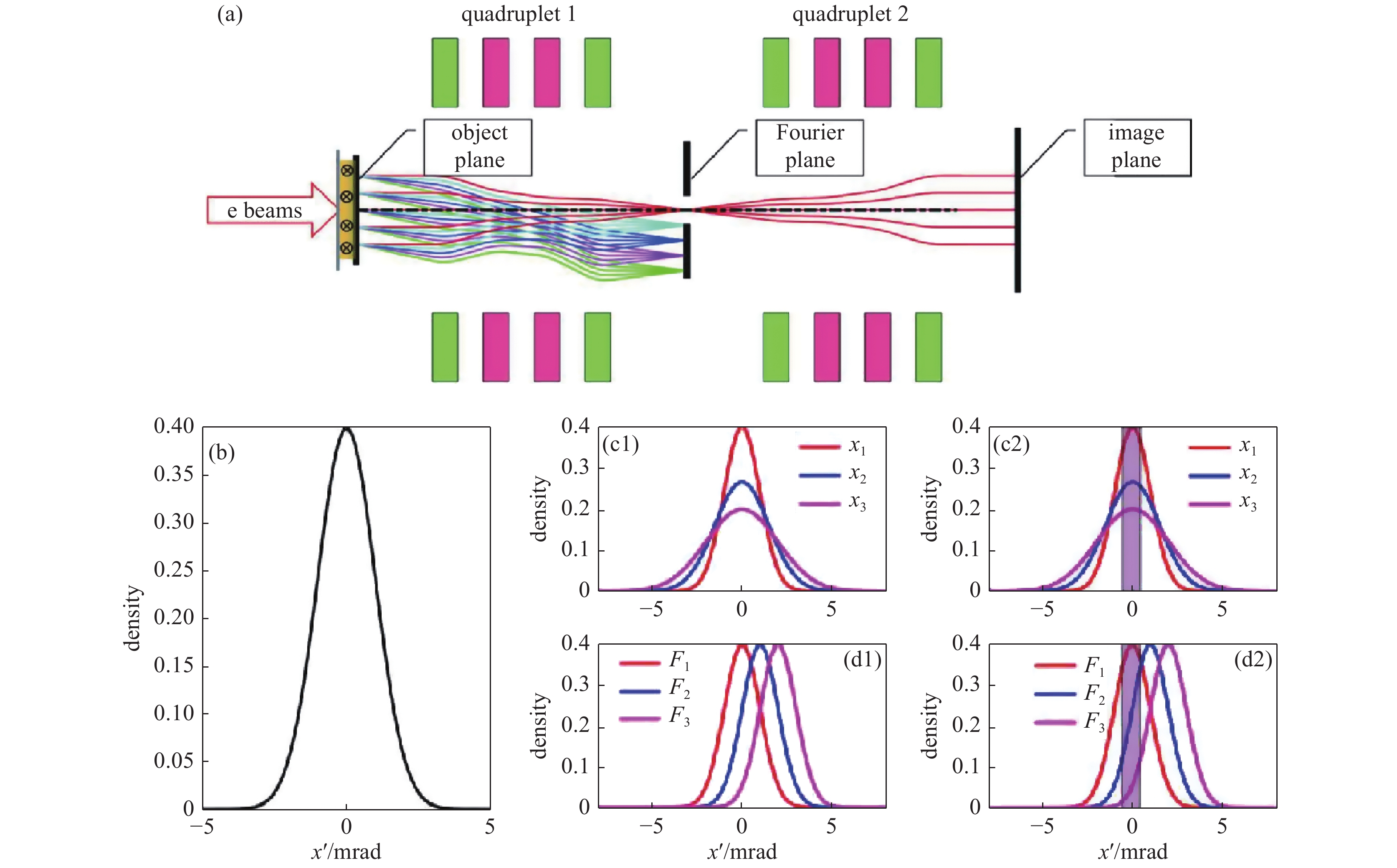
It means that the electron angle information at the object plane has been translated into the position information at this plane. An aperture at this plane can achieve angle selection for passing electrons. The principle schematic is shown in Fig.1.

In the x-axis direction, the spatial resolution is $ \mathrm{\Delta }{x}_{i}={R}_{12}{x}_{0}'+{T}_{126}{x}_{0}'\delta +{T}_{116}{x}_{0}\delta $, $ {T}_{126} $ and $ {T}_{116} $ are the second order terms of transport matrix, $ \delta $ is the energy spread of electron beam. Since R₁₂ is close to zero and the energy spread is mainly from bremsstrahlung for high energy electrons, this method is limited for thin or low z target diagnosis. In this case, the transmittance of electrons after penetrating the specimen is about 1. When we set an aperture at the Fourier plane, the transmittance after it can be described as ${T}_{{\rm{r}}}(\theta ,t)={\displaystyle\int }_{-\varepsilon }^{\varepsilon }g(\varphi -\theta ,t)\mathrm{d}{x}_{0}'$, where $ \varepsilon =\dfrac{w}{2{R}_{12\mathrm{F}}} $, and $ w $ is the aperture size.

In view of the above analysis, the transmittance of monoenergetic electron beams is dominated by three factors, which are the matter areal density, the E/B field strength and the aperture size. For the multiple degrees of freedom diagnosis, more equations are necessary. In single shot experiment, the aperture size is unchangeable, and θ is difficult to modulate. Modulating the thickness of the specimen is an effective way to get a set of equations. This can be achieved by adopting a premodulation grille scattering target before the diagnosed target. A grille target example is shown in Fig.2(a).

With the grille scattering target, two transmittance values can be obtained for each image point in single radiography. One is the measured one, the other is got from fitting the neighbor area, which has different areal density at the scattering target. The corresponding transmittances at the image plane can be denoted by T_r(t+t₁,θ) and T_r(t+t₂,θ), where t is the relative thickness of the diagnosed target, t₁ and t₂ are the two relative thicknesses of the grille scattering target. With the two equations, t and θ can be solved within a certain range. The principle is shown in Fig.2(b).

Extend to two-dimensional plane, the transmittance density can be described as^[24]

$ j({x}_{0}',{y}_{0}',t)=f({\rho }',{\varphi }',t)=f\Bigg(\sqrt{{x}_{0}'^{2}+{y}_{0}'^{2}},{\varphi }',t\Bigg) $ (5)

where $ {\rho }' $, ${\varphi }'$ are the polar coordinates. With the aperture’s selection, the transmittance can be described by the following formula:

$ {T}_{{\rm{r}}}(t,\boldsymbol{\theta })=\iint\nolimits_{({\rho }',{\varphi }')\in {S}'} f({\rho }',{\varphi }',t){\rho }'\mathrm{d}{\rho }'\mathrm{d}{\varphi }' $ (6)

where $ {S}' $ refers to the aperture gating area. When the aperture is set as an ellipse shape, and the half-axis satisfies $ \dfrac{{l}_{x}}{{l}_{y}}=\dfrac{{R}_{12\mathrm{F}}}{{R}_{34\mathrm{F}}} $, the transmittance can be described by

$ \left\{ \begin{array}{l} {T}_{{\rm{r}}}(t,\boldsymbol{\theta })={\displaystyle\int }_{0}^{\varepsilon }{\displaystyle\int }_{0}^{2\mathrm{\pi }}{f}_{t}\left({\rho }_{t}'\right){\rho }'\mathrm{d}{\rho }'\mathrm{d}{\varphi }'\\ \dfrac{{l}_{x}}{{R}_{12\mathrm{F}}}=\dfrac{{l}_{y}}{{R}_{34\mathrm{F}}}=\varepsilon \end{array} \right.$ (7)

where $ {f}_{{\rm{t}}} $ is the transmittance density when there is only matter and no E/B field in the target, and $\; {\rho }_{{\rm{t}}}' $ is the radius with the center of $ f({\rho }',{\varphi }',t) $ as the pole, and

$ {\rho }_{{\rm{t}}}'=\sqrt{{({\rho }'\mathrm{c}\mathrm{o}\mathrm{s}{\varphi }'-{\rho }_{\boldsymbol{\theta }}')}^{2}+{\left({\rho }'\mathrm{s}\mathrm{i}\mathrm{n}{\varphi }'\right)}^{2}} $ (8)

${\rho }_{\boldsymbol{\theta }}'$ is the shift distance caused by E/B field. There isn’t any factor related to the direction of the shift caused by E/B in Eq.(8), which indicates that the transmittance is independent of the direction of $ \boldsymbol{\theta } $.

When the aperture is set as a ring, the inner and outer radii satisfy $ \dfrac{{l}_{{\rm{i}}x}}{{R}_{12\mathrm{F}}}=\dfrac{{l}_{{\rm{i}}y}}{{R}_{34\mathrm{F}}}={\varepsilon }_{1} $ and $ \dfrac{{l}_{{\rm{o}}x}}{{R}_{12\mathrm{F}}}=\dfrac{{l}_{{\rm{o}}y}}{{R}_{34\mathrm{F}}}={\varepsilon }_{2} $, and the transmittance can be described by

$ {T}_{{\rm{r}}}(t,{\boldsymbol{\theta}} )={\displaystyle\int }_{{\varepsilon }_{1}}^{{\varepsilon }_{2}}{\displaystyle\int }_{0}^{2\mathrm{\pi }}{{{f}}}_{{\rm{t}}}\left({\rho }_{{\rm{t}}}'\right){\rho }'\mathrm{d}{\rho }'\mathrm{d}{\varphi }' $ (9)

The transmittance will still be independent of the direction of $ \boldsymbol{\theta } $.

In two-dimensional plane, we can set a pre-modulation scattering target with four thicknesses before the real diagnosed target, as shown in Fig.3(a). Fig.3(b) is the front view of a scattering target example.

Thus, four transmittance values can be obtained for each point at the image plane. The first one is the measured one, the other three transmittances is derived from fitting and interpolating the transmittance along the three lines in Fig.3(b). Finally, four equations can be obtained as Eq.(10), which is more than enough to give a precise solution of t and $ \theta $ in a specific range.

$ \left\{\begin{array}{c}{T}_{{\rm{r}}1}={T}_{{\rm{r}}}(t+{t}_{1},\theta )\\ \begin{array}{c}{T}_{{\rm{r}}2}={T}_{{\rm{r}}}(t+{t}_{1},\theta )\\ {T}_{{\rm{r}}3}={T}_{{\rm{r}}}(t+{t}_{1},\theta )\\ {T}_{{\rm{r}}4}={T}_{{\rm{r}}}(t+{t}_{1},\theta )\end{array}\end{array}\right. $ (10)

To analyze the feasibility of this method, we simulated 50 MeV electrons diagnosing hydrogen and E/B field. To make the areal density and E/B field have independence in separate dimensions, we set the diagnosed sample as Fig.4(a).

The sample was set as a wedge shape. Considering the diagnosis ability of 50 MeV electron beams, we set the areal density of hydrogen increasing from 0.5 mg/cm² to 5.5 mg/cm² along the x-axis and the density was 1 g/cm³, θ was decreasing from 5 mrad to 0 mrad along the y-axis. We tried a set of scattering target thicknesses, 0 µm, 2 µm, 4 µm and 8 µm, for contrast, so there were $ {C}_{4}^{2} $ combinations of thicknesses. The EGS5 code^[25] was used to simulate the beam target interaction, and the beam optics was considered ideally. Fig.5 and Fig.6 show the analysis results when the aperture is set as an ellipse hole and a ring as presented in Fig.4(b) and (c) respectively.

As shown in Fig.5(a), for the transmittance of a point at the image plane, there will be a corresponding contour line with X-θ as variables. Draw the contour lines with different scattering target thicknesses in one picture, as illustrated in Fig.5(b), there will be an intersection point between the two contour lines with the same transmittance, which indicates the solution (X, θ). The resolution of X and θ is better in larger θ area. In lower θ area, the contour lines are almost parallel. This indicates that this design is suitable for diagnosing the fluid in strong E/B field. Meanwhile, compare different combinations in Fig.5(b), it can be concluded that the larger the difference of scattering target thicknesses is, the better resolution of (X,θ) we can get. In other words, contour lines of 0 µm and 8 µm are the better choice to fix the solution (X, θ). The other two thicknesses can improve the E/B field diagnosis range. When the aperture is set as an ellipse hole, as mentioned above, the resolution will deteriorate in low θ area. To solve this problem, a ring aperture as Fig.4(c) demonstrates, which sets the angle acceptance as (1,2) mrad, is adopted. The analysis results are shown in Fig.6.

In Fig.6(a), when the angle acceptance range is set to (1, 2) mrad, the transmittance distributions have obviously been changed. Compare Fig.6(b) with Fig.5(b), the resolution at low θ area is improved a lot. On the other hand, two contour lines with the same transmittance in Fig.6(b) could have two intersection points, which correspond to two different solutions (X₀₁, θ₀₁) and (X₀₂, θ₀₂). Under such circumstances, a third contour line from different scattering target thickness but with the same transmittance can help to make the solution settled.

In summary, the areal density difference diagnostic method based on HEELR is proposed to make dual degrees of freedom consists of areal density and E/B field strength diagnosis in this paper. In two-dimensional plane, four transmittances from different scattering target thicknesses can be obtained. When the angle acceptance area of the beam line is a circle, this method is suitable for the diagnosed system with strong E/B field. When the aperture is set as a ring, the effective diagnostic range can be extended to the low E/B field area. In an actual experiment, we need to adjust the scattering target thickness, the aperture shape and size, even the incident beam energy to match different diagnosed system. Furthermore, since this method can provide four equations, the vector of field and another degree of freedom may be obtained, just like the coupling in the strong coupled system diagnosing.

References

[1] Walsh C A, Chittenden J P, McGlinchey K, et al. Self-generated magnetic fields in the stagnation phase of indirect-drive implosions on the National Ignition Facility[J]. Physical Review Letters, 118, 155001(2017).
[2] Fox W, Bhattacharjee A, Germaschewski K. Magnetic reconnection in high-energy-density laser-produced plasmas[J]. Physics of Plasmas, 19, 056309(2012).
[3] Gotchev O V, Chang P Y, Knauer J P, et al. Laser-driven magnetic-flux compression in high-energy-density plasmas[J]. Physical Review Letters, 103, 215004(2009).
[4] Lindemuth L R, Ekdahl C A, Fowler C M, et al. US/Russian collaboration in high-energy-density physics using high-explosive pulsed power: ultrahigh current experiments, ultrahigh magnetic field applications, and progress toward controlled thermonuclear fusion[J]. IEEE Transactions on Plasma Science, 25, 1357-1372(1997).
[5] Merrill F E, Campos E, Espinoza C, et al. Magnifying lens for 800 MeV proton radiography[J]. Review of Scientific Instruments, 82, 103709(2011).
[6] Kantsyrev A V, Golubev A A, Bogdanov A V, et al. TWAC-ITEP proton microscopy facility[J]. Instruments and Experimental Techniques, 57, 1-10(2014).
[7] Rygg J R, Séguin F H, Li C K, et al. Proton radiography of inertial fusion implosions[J]. Science, 319, 1223-1225(2008).
[8] Tommasini R, Landen O L, Hopkins L B, et al. Time-resolved fuel density profiles of the stagnation phase of indirect-drive inertial confinement implosions[J]. Physical Review Letters, 125, 155003(2020).
[9] Martynenko A S, Pikuz S A, Skobelev I Y, et al. Optimization of a laser plasma-based X-ray source according to WDM absorption spectroscopy requirements[J]. Matter and Radiation at Extremes, 6, 014405(2021).
[10] Zhao Yongtao, Zhang Zimin, Gai Wei, et al. High energy electron radiography scheme with high spatial and temporal resolution in three dimension based on a e-LINAC[J]. Laser and Particle Beams, 34, 338-342(2016).
[11] Xiao Jiahao, Zhang Zimin, Cao Shuchun, et al. Areal density and spatial resolution of high energy electron radiography[J]. Chinese Physics B, 27, 035202(2018).
[12] Wang Feng, Jiang Shaoen, Ding Yongkun, et al. Recent diagnostic developments at the 100 kJ-level laser facility in China[J]. Matter and Radiation at Extremes, 5, 035201(2020).
[13] Li C K, Séguin F H, Frenje J A, et al. Measuring
[14] Li C K, Séguin F H, Frenje J A, et al. Monoenergetic-proton-radiography measurements of implosion dynamics in direct-drive inertial-confinement fusion[J]. Physical Review Letters, 100, 225001(2008).
[15] Liao Guoqian, Li Yutong, Zhu Baojun, et al. Proton radiography of magnetic fields generated with an open-ended coil driven by high power laser pulses[J]. Matter and Radiation at Extremes, 1, 187-191(2016).
[16] Schumaker W, Nakanii N, McGuffey C, et al. Ultrafast electron radiography of magnetic fields in high-intensity laser-solid interactions[J]. Physical Review Letters, 110, 015003(2013).
[17] Zhu P F, Zhang Z C, Chen L, et al. Ultrashort electron pulses as a four-dimensional diagnosis of plasma dynamics[J]. Review of Scientific Instruments, 81, 103505(2010).
[18] Li Junjie, Wang Xuan, Chen Zhaoyang, et al. Ultrafast electron beam imaging of femtosecond laser-induced plasma dynamics[J]. Journal of Applied Physics, 107, 083305(2010).
[19] Chen Long, Li Runze, Chen Jie, et al. Mapping transient electric fields with picosecond electron bunches[J]. Proceedings of the National Academy of Sciences of the United States of America, 112, 14479-14483(2015).
[20] Merrill F, Harmon F, Hunt A, et al. Electron radiography[J]. Nuclear Instruments and Methods in Physics Research Section B: Beam Interactions with Materials and Atoms, 261, 382-386(2007).
[21] Merrill F E, Goett J, Gibbs J W, et al. Demonstration of transmission high energy electron microscopy[J]. Applied Physics Letters, 112, 144103(2018).
[22] Zhou Zheng, Fang Yu, Chen Han, et al. Visualizing the melting processes in ultrashort intense laser triggered gold mesh with high energy electron radiography[J]. Matter and Radiation at Extremes, 4, 065402(2019).
[23] Xiao Jiahao, Du Yingchao, Zhang Shizheng, et al. Ultrafast high-energy electron radiography application in magnetic field delicate structure measurement[J]. Laser and Particle Beams, 6683245(2021).
[24] Xiao Jiahao, Du Yingchao, Li Haoqing, et al. Ultrafast high energy electron lens radiography suitable f transient electromagic field diagnosis [J]. Journal of Instrumentation, 2022, 17(01):P01033 DOI:10.1088174802211701P01033
[25] Hirayama H, Namito Y, Bielajew A F, et al. The EGS5 code system[R]. SLACR730, 2005.
Set citation alerts for the article
Please enter your email address
© Copyright 2018-2021 | Chinese Laser Press. All Rights Reserved 沪ICP备15018463号-20