Deep reinforcement with spectrum series learning control for a mode-locked fiber laser

Zhan Li; Shuaishuai Yang; Qi Xiao; Tianyu Zhang; Yong Li; Lu Han; Dean Liu; Xiaoping Ouyang; Jianqiang Zhu

doi:10.1364/PRJ.455493

Abstract

A spectrum series learning-based model is presented for mode-locked fiber laser state searching and switching. The mode-locked operation search policy is obtained by our proposed algorithm that combines deep reinforcement learning and long short-term memory networks. Numerical simulations show that the dynamic features of the laser cavity can be obtained from spectrum series. Compared with the traditional evolutionary search algorithm that only uses the current state, this model greatly improves the efficiency of the mode-locked search. The switch of the mode-locked state is realized by a predictive neural network that controls the pump power. In the experiments, the proposed algorithm uses an average of only 690 ms to obtain a stable mode-locked state, which is one order of magnitude less than that of the traditional method. The maximum number of search steps in the algorithm is 47 in the 16°C–30°C temperature environment. The pump power prediction error is less than 2 mW, which ensures precise laser locking on multiple operating states. This proposed technique paves the way for a variety of optical systems that require fast and robust control.

1. INTRODUCTION

The all-normal dissipative (ANDi) soliton mode-locked fiber laser based on the nonlinear polarization evolution (NPE) mechanism [1,2] has been applied in several scientific fields, such as high-power laser research [3] and two-photon microscopy [4], owing to its simple structure and high single-pulse energy. However, the cavity parameters of this laser are sensitive to environmental changes, resulting in changes in the mode-locked operation state. Strict fixation of the fiber and environmental shielding are required to achieve stable operation of the laser, limiting its application. To improve the robustness of the mode-locked fiber laser, various algorithms based on the evolutionary algorithm and adaptive control have been adapted to drive the electric polarization controller (EPC), making the laser self-tuning [5 –7]. However, the current control policy considers mode-locked searching only as an optimization problem and accelerates it using well-designed loss functions and special feedback loops. The physical mechanism of the mode-locked process has not been considered, making it difficult to establish the mapping from the laser output to the EPC state.

The generation of ANDi pulses depends on the balance of dispersion, gain, loss, and self-phase modulation (SPM) in the fiber cavity. Maintaining this balance is a process of evolutionary propagation that exhibits high time dependence [8 –10]. That means it is natural to choose a model that can use time-series features to make decisions, rather than relying only on current observations. On the other hand, the key aspect of the self-tuning NPE-based mode-locked laser is the search for an appropriate operating point in the cavity to realize a mode-locked state switch. An intelligent algorithm in a specific environment (fiber laser) needs to learn the high-dimensional characteristics of the environment after sufficient exploration in the initial stage, so that the next action can be directly obtained based on previous experience and current observations. A learning-based neural network is a solution to these problems [11 –13]. In particular, deep reinforcement learning (DRL) [14 –16] has been applied in complex system control for photonics research owing to its powerful high-dimensional feature analysis ability. For mode-locked fiber laser control, neural networks have also been used to predict cavity parameters based on numerical simulations [15]. DRL is also applied into mode-locked control by using deep $Q$ -learning (DQN) [17] and deep deterministic policy gradient (DDPG) [18]. These DRL algorithms are suitable for constant environments only; retraining is required if the environment changes. Therefore, it is necessary to build a network that truly learns the essence of mode-locked state adjusting to control the laser state in a changing environment.

In this study, a mode-locked operating mode search (MDRL) and a switching algorithm (MSP) are proposed based on DRL and spectrum series learning. The dynamic process of mode-locked evolution is related to the state of the last pulse. A physical map is established between the input spectrum and the EPC state of the output by extracting the associated features of the time series and introducing spectral information, and it greatly improved the search efficiency. The performance and robustness of the proposed method are demonstrated both theoretically and experimentally. This method is capable of reaching the mode-locked state from a random state in fewer search steps than the previously reported method [5 –7].

Sign up for Photonics Research TOC. Get the latest issue of Photonics Research delivered right to you！Sign up now

2. METHODS

A. Feedback Time-Series Spectrum Control Model

For a typical mode-locked fiber laser, the pulse evolution in the fiber can be described by the Schrödinger equation [19,20]. In the Fourier domain, it can be written as $\frac{d}{d z} A (z, ω) + (\frac{α}{2} - \frac{i β_{2}}{2} ω^{2} + \frac{i β_{3}}{6} ω^{3}) A (z, ω) = i γ {| A (z, ω) |}^{2} A (z, ω),$ (1)where $A (z, ω)$ is the electric field envelope, $ω$ is the angular frequency, $z$ is the propagation coordinate, $α$ is the fiber loss, $β_{2}$ and $β_{3}$ are the second-order and third-order dispersion, respectively, and $γ$ is the nonlinear refractive index of the fiber. This indicates that the state of the pulse in the Fourier domain is a serialization process, and the spectrum $| A (ω, z) |$ is highly correlated with the electric field $A (ω, 0)$ . To illustrate the effectiveness of the time-series control, Eq. (1) is used to trace the evolution of the pulse in a typical dissipative soliton mode-locked laser based on NPE [21], with element parameters identical to those in the Section 3. To simplify the calculation, the amplitude modulation mechanism of the NPE is considered equivalent to the transmittance of a fast saturable absorber [22,23]. In the simulation, we defined two NPE states: the low loss transmission state $T_{L}$ and high loss transmission state $T_{H}$ . The transmittance of the amplitude modulation generated in the cavity is shown in Fig. 1(d).

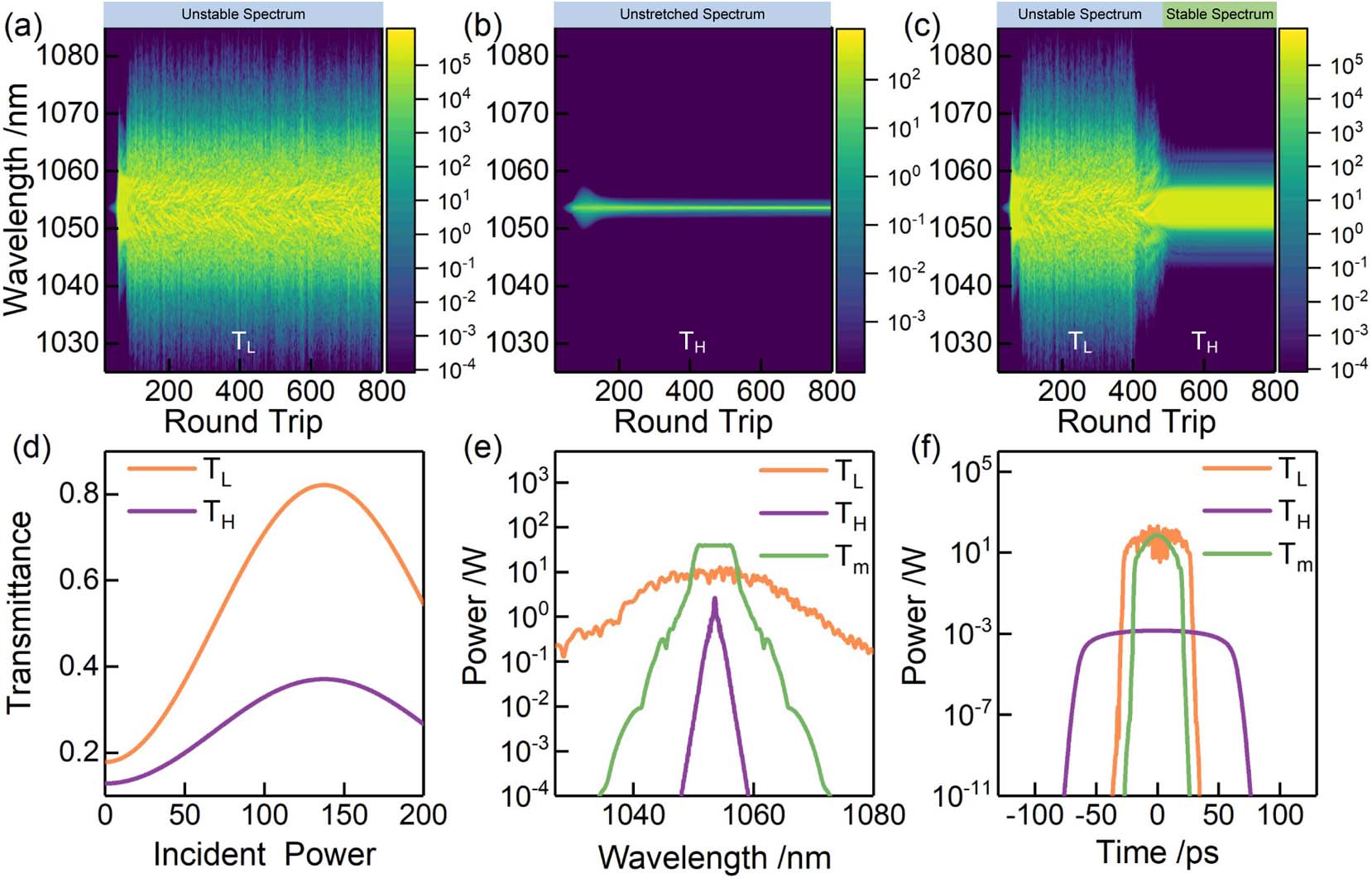
Figure 1.GNLSE simulation result from the NPE-based mode-locking laser system. (a) Spectral evolution when EPC is in $T_{L}$ . (b) Spectral evolution when EPC is in $T_{H}$ . (c) Spectral evolution when EPC is in $T_{L}$ initially and then converted to $T_{H}$ after 400 round trips. (d) Light transmittance caused by NPE when EPC is in $T_{L}$ (orange line) and $T_{H}$ (purple line). (e) Spectrum output after 800 round trips when EPC is in $T_{L}$ (orange line), $T_{H}$ (purple line), and $T_{m}$ (green line). (f) Temporal output after 800 round trips when EPC is in $T_{L}$ (orange line), $T_{H}$ (purple line), and $T_{m}$ (green line).

When the laser is in the $T_{L}$ state, the higher peak power part of the pulse corresponds to the larger nonlinear phase shift, which can yield higher transmittance. The spectrum evolution for this state is shown in Fig. 1(a). The pulse spectrum is rapidly expanded and amplified during the first 35 round trips, establishing a mode-locked state. Subsequently, owing to the low loss in the cavity, an excessive nonlinear phase shift is introduced, which decreases the NPE transmittance and causes pulse splitting. In this state, the pulse cannot maintain a stable mode-locked output, and the final output spectral and time waveforms are shown as orange lines in Figs. 1(e) and 1(f). In the $T_{H}$ state, because of the low transmittance, the pulse portion of the peak power does not increase its gain sufficiently, and the spectrum of the pulse cannot be sufficiently stretched and amplified, as shown in Fig. 1(b). As shown by the purple line in Figs. 1(e) and (f), with a round trip increase, the pulse is only stretched by the fiber group velocity dispersion, and such a low peak power cannot form an effective output.

In the traditional mode-locked search algorithm [7], the above two EPC states are considered to be unable to obtain an effective mode-locked state. However, if combined with two states as a time-series control $T_{m}$ , the low loss state is used to expand and amplify the pulse spectrum sufficiently. Then, $T_{H}$ is introduced to reduce the SPM effect and obtain a stable mode-locked output with high peak power. The spectrum evolution is shown in Fig. 1(c); in the first 400 round trips, EPC is in $T_{L}$ , and similarly to Fig. 1(a), the spectrum of the pulse is amplified, broadened, and split. After that, the EPC state is changed to high loss, the splitting pulse is rapidly suppressed, and the remaining pulse spectrum is expanded to obtain a stable mode-locked output, as shown by the green line in Figs. 1(e) and 1(f). Therefore, considering the influence of the previous spectrum distribution, time-series control can make more effective decisions and greatly improve the search efficiency.

This illustrates that the NPE-based mode-locked laser output spectrum depends on the previous spectral distribution and polarization modulation by the EPC. However, the shape of the spectrum is difficult to quantify with simple features, and conventional time-series feature extraction requires statistical or wavelet analysis for each time segment [24], which is inefficient and difficult to generalize. Long short-term memory (LSTM) is an architecture of recurrent neural networks, and at each time step, the output is connected cyclically to the hidden unit of the next time step [25]. The gate cell of LSTM solves the problem of gradient vanishing caused by the long-term dependence of time-series data. This approach has been applied successfully to speech recognition [26], machine translation [27], and other sequential tasks. These characteristics make LSTM suitable for analyzing and predicting the dynamic process of spectrum variation in mode-locked lasers [28].

After the spectral series features are obtained, a model is still needed to map the input spectral signal to the output EPC driver signal to make the laser self-tuning. Recently, combined with deep learning, DRL has made great progress in complex tasks that are unreachable for conventional optimization algorithms, especially to solve the sequential decision-making problem under uncertainty [14,17,18]. To apply the time-series spectrum control to the ANDi laser, we have proposed a novel feedback control model, which is shown in Fig. 2.

Figure 2.Feedback time-series spectrum control model.

This model consists of two parts, which are the mode-locked deep reinforcement learning (MDRL) agent and the mode-locked state prediction (MSP) network, and these network structures are described in detail in Section 2.B. The fiber laser has two controlled objects: the polarization controller position and the pump power. At first, the pump power of the fiber laser is set to an appropriate point. By extracting the time-series spectral features of fiber laser, MDRL can search for the best position of polarization controller, so that the laser can reach a stable fundamental mode-locked state from an arbitrary initial state. After MDRL searching, the polarization controller position is fixed to constant. From the output spectrum, it is difficult to quantify the differences between mode-locked states from the spectral distribution by using simple low-dimensional features. We use the MSP net starts to learn the map from the laser output spectrum to the pump power. The well-trained MSP network is used to realize mode-locked state switches by controlling the laser pump power.

B. Mode-Locked Deep Reinforcement Learning Agent

Reinforcement learning has two main components: the environment and the agent make up a Markov process [16]. The agent learns the action $a_{t}$ based on the current environment observation $s_{t}$ to maximize its cumulative reward $R$ . At each step, the environment provides $s_{t}$ and $R$ when the last action $a_{t - 1}$ acts upon it. A common DRL architecture is actor–critic (AC) [16,29], in which the actor is a policy network $π (s_{t})$ to choose $a_{t}$ based on $s_{t}$ , and the critic refers to the estimation of the value network $V (s_{t})$ . Based on the AC framework and neural network, we establish a novel reinforcement model, MDRL, shown in Fig. 3, which uses an actor network and a critic network to represent $π (s_{t})$ and $V (s_{t})$ , respectively. The environment is the NPE-based mode-locked fiber laser, the input observation $s_{t}$ represents the data from the optical spectrum analyzer, and the action $a_{t}$ consists of four channels of voltage data for the EPC to control the polarization modulation, and thus generate the NPE in the fiber cavity.

Figure 3.MDRL agent layout.

Because the EPC control voltages are continuous, $a_{t}$ will have a continuous action space, making uncertainty typically grow in direct action prediction. Therefore, the diagonal Gaussian policy [30] is chosen to regress the distribution of $a_{t}$ in the actor network, which has a mean value path $μ_{θ} (s_{t})$ and a standard deviation path $σ_{θ} (s_{t})$ from the data after the actor network pipeline process. $a_{t}$ is computed using $a_{t} = π (s_{t}) = μ_{θ_{π}} (s_{t}) + σ_{θ_{π}} (s_{t}) \cdot z,$ (2)where $t$ is the current step, $\cdot$ is an element-wise product, $θ_{π}$ represents the parameters of the current actor network, and $z$ is a Gaussian noise term. In the critic network, the expected cumulative return $V (s_{t} | θ_{V})$ is estimated by two fully connected layers after the pipeline process, where $θ_{V}$ represents the parameters of the critic network.

As shown in the Fig. 3, both the actor network and the critic network first require a pipeline process for mapping input optical spectrum data into high-dimensional space and extracting the features from time series. The pipeline includes a full connection layer, an LSTM layer, and a dropout layer. The dropout layer is used to reduce the overfitting of the network during training. In the networks, each full connection and LSTM layer are activated by an ReLU function [31].

The target of the reinforcement learning agent is to maximize the expected cumulative reward $R$ for each episode. Reward shaping [32] is used to reduce the decrease in learning efficiency owing to the sparse mode-locked state in the entire search space. The final reward is $R (w_{t}) = {\begin{cases} ReLU (w_{t} - w_{t - 1}), & w_{t} < w_{G} \\ w_{t}^{2} + α (T - t) + \frac{w_{t}}{w_{rise, t}}, & w_{t} \geq w_{G} \end{cases},$ (3)where $w_{t}$ is the full width at half maximum (FWHM) of $s_{t}$ , also known as the spectrum width, $ReLU$ is the rectified linear unit operator [31], $w_{G}$ is the threshold of $w_{t}$ , $T$ is the total number of search steps in each episode, $α$ is the discount factor, and $w_{rise, t}$ is the rising edge width. In mode-locked laser state switching, $w_{t}$ of the free-run state is less than that of the mode-locked state, so when $w_{t} < w_{G}$ , the laser state is considered to be free run. The agent uses the increase in $w_{t}$ as the reward function to make the reward in the search space relatively dense, and searching is performed in the direction of increasing $w_{t}$ . In addition, the ReLU operator is added to ensure non-negative output. When $w_{t} \geq w_{G}$ , the laser is in a mode-locked state, $w_{t}^{2}$ guarantees a sufficient reward of $a_{t - 1}$ , and $α (T - t)$ is used to minimize the number of search steps in one episode. $w_{t} / w_{rise, t}$ is used to reduce the width of the rising edge because the dissipative soliton mode-locked laser output is a pulse that has a sharp optical spectrum edge, and a smooth $w_{rise, t}$ will induce an unstable pulse. In the experiment $w_{G} = 3 nm$ (spectrum width), $α = 0.1$ .

In the agent training, each episode has two stages: sampling and learning. In the sampling stage, the agent samples the environment $N$ times according to the current parameters $θ_{π}, θ_{V}$ . At each sampling step, the estimated return $G_{t}$ is computed using Eq. (4), following the asynchronous advantage actor–critic model: $G_{t} = \sum_{i = t}^{N} γ^{i - t} R_{i} + γ^{N - t} V (s_{N} | θ_{V}),$ (4)where $N$ is the number of environment samples, $γ$ is the discount factor, $θ_{V}$ holds the current parameters of the critic network, and $s_{N}$ is the $N_{th}$ environment observation. The data ${s_{t}, a_{t}, G_{t}}$ are stored in the reply memory. After environment sampling, the data in the reply memory are used as the training set to train and update the parameters of the actor and critic neural networks.

In contrast to general deep learning training methods, reinforcement learning networks cannot use the truth value directly to train the network because the environment is unknown. Therefore, it is necessary to design the loss function carefully to maximize $G_{i}$ of the current policy. In MDRL, the critic network and actor network training losses are defined by proximal policy optimization (PPO) [33] to improve the agent training efficiency and avoid training failure caused by use of the wrong training set. The critic network loss function is $L_{critic} = \frac{1}{M} \sum_{i = 1}^{M} {(G_{i} - V (s_{i} | θ_{V}))}^{2},$ (5)where $M$ is the mini-batch size. The actor network loss function is $L_{actor} = - \frac{1}{M} \sum_{i = 1}^{M} (r_{t} (θ_{π}) A_{i}, clip (r_{t} (θ_{π}),1 - ϵ,1 + ϵ) A_{i}),$ (6)where $A_{i} = G_{i} - V (s_{i} | θ_{V})$ , $r_{t} = \frac{π_{θ} (s_{t})}{π_{θ_{old}} (s_{t})}$ is the probability ratio, the clip function clip constrains $r_{t} (θ_{π})$ into $[1 - ϵ, 1 + ϵ]$ , and $ϵ$ is the clip factor. After obtaining $L_{actor}, L_{critic}$ , and error backpropagation, the actor and critic network parameters are updated by Adam optimization. In the learning stage, the agent has trained over $K$ epochs and then starts a new episode, until the search reaches the maximum number of episodes.

C. Mode-Locked State Prediction Network

In a certain environment, as the pump power gradually increases, the output of the mode-locked pulse evolves from free-running, through Q-switching (QS) and Q-switched mode-locked (QML), to the fundamental mode-locked (FML) state [34]. In addition, the output spectrum will also transform from a single-mode output to a stable wide mode-locked spectrum. If the pump power continues to increase, the spectrum will broaden gradually owing to SPM until the pulse splits into higher-order solitons, resulting in a harmonic mode-locked (HML) state. However, different mode-locked states have different spectral distributions. Moreover, there is no effective method to describe the spectral differences in different mode-locked states. However, deep learning has a powerful feature description ability that can classify signals in a high-dimensional space. Therefore, we have established an MSP neural network based on a convolutional neural network.

In the prediction network, the spectrum signal is first sent to five Conv-Blocks to extract the signal features, and each Conv-Block has a convolution layer, a batch normalized layer, and an ReLU layer. Then, after fully connected layer preprocessing, the features are handled by two paths. In the classification path, the softmax layer is used to map the spectrum features to the mode-locked state. In the prediction path, the fully connected layer is used to predict the current pump power.

D. Neural Network Implementation and Training

Under the actual NPE-based laser environment, both the MDRL agent and MSP are implemented based on version 1.1.0 of the PyTorch platform using Python 3.6.4, running on a computer with two NVIDIA TITAN RTX GPUs with 64 GB of memory. The MDRL agent is trained for 5000 episodes, and the maximum number of steps in the search stage of one episode is 400. After the search stage, the Adam optimizer with a learning rate of 0.001 updates the weights and biases of the networks for 10 epochs. In our study, the input spectrum from the optical spectrum analyzer is cropped to the range from 1030 nm to 1080 nm with a resolution of 0.1 nm. The agent output consists of four channels of voltage data ranging from 22,125 V to 5 V, to control the EPC to produce different polarization modulations. The total training time is $\sim 3 h$ under a 3000 mW pump power environment.

After MDRL obtained a stable mode-locked state, we controlled the pump power to increase linearly from 40 mW to 420 mW, with a 1 mW stepping value, and recorded 200 spectral images at each voltage as the input training dataset for MSP. At the same time, the distribution of pulse sequences was observed using an oscilloscope to determine the current mode-locked state. The MSP has two output channels: the mode-locked state and the pump power. Therefore, the output of the MSP training dataset is the set of the current pump power and the current mode-locked state. After obtaining the training dataset, the MSP network was trained for 200 epochs using the same optimizer as MDRL, with a learning rate of 0.01. The cross-entropy loss function and smooth $L_{1}$ loss function [35] are used to train the classification path and the regression path, respectively.

3. RESULTS

Figure 4 shows the layout of the reinforcement learning environment, which is a dispersion soliton fiber laser with a center wavelength of 1053 nm. The fiber section consists of $\sim 15 m$ single-mode fiber (SMF) and $\sim 0.3 m$ ytterbium-doped fiber (YDF). The SMF has 2.1 dB/km attenuation and 6.2 μm mode field diameter (MFD), the YDF has 25.6 dB/km attenuation and 4 μm MFD, and the total dispersion is $0.338 {ps}^{2}$ . $\sim 250 mW$ LD with a center wavelength of 980 nm is coupled to the core of the YDF by a wavelength division multiplexer (WDM). NPE is implemented by EPC (OZ Optics EPC-400), an isolator I, and a polarizer P. After passing through P, a random noise pulse is polarized in a certain direction and then converted to an elliptically polarized state. The nonlinear phase shift generated by SPM in the fiber is converted to amplitude modulation in P to produce saturable absorption [22]. The EPC, which is used to generate NPE, can produce a state of polarization (SOP) located at an arbitrary position of the Poincaré sphere in the SMF. By inputting four channel voltages, this component can precisely manipulate the NPE process and realize simple and efficient control of the operating state in the cavity. A spectrum filter SF with 1053 nm center wavelength and 10 nm bandwidth is added after EPC1 to suppress the emission peak at 1030 nm and improve mode-locked stability [21]. The output mode-locked pulse is coupled by C2, and 1% output power is delivered into a diagnostic optical spectrum analyzer D (Ocean Insight USB4000) to monitor the spectrum change of the mode-locked pulses and send spectrum data as observations to the MDRL agent.

Figure 4.MDRL environment layout. LD, laser diode; WDM, 980/1060 nm wavelength division multiplexer; YDF, ytterbium-doped fiber; C, coupler; SMF, single-mode fiber; P, polarizer; I, isolator; EPC, electrical polarization controller; SF, optical spectrum filter; D, diagnostic optical spectrum analyzer.

In the experiment, the pump power is first fixed at 300 mW and then begins MDRL agent training. Each search step of the MDRL agent costs $\sim 50 ms$ , including $\sim 10 ms$ spectrum analyzer exposure time and $\sim 40 ms$ communication and computation time. Using the well-trained MDRL agent, the mode-locked state can be searched at a 20 Hz control frequency starting from arbitrary initial EPC voltages. We first set EPC voltages to four random values and run the MDRL agent to obtain an FML state. The spectrum and time-wave evolution data that are acquired from D and an oscilloscope (TELEDYNE Lecroy WaveMaster 813Zi-B) are shown in Figs. 5(a) and 5(b). In the FML state, the average output power is 37 mW, the repetition rate is 13.5 MHz, the center wavelength is 1053 nm, the spectrum bandwidth is 8.5 nm, and the pulse output width is 14.2 ps. Since the ANDi laser has no dispersion management in the cavity, the output pulse is highly chirped [1] as shown by the blue line in Fig. 5(d). Grating pairs are used to compensate for the dispersion of the pulses outside the cavity, and the measured autocorrelation results of the pulses are shown in Fig. 5(d). The autocorrelation width of 272 fs fitted by ${sech}^{2}$ is converted to the pulse width of $\sim 176.6 fs$ , which is close to the Fourier transform limit [36,37].

Figure 5.Spectrum and time-wave evolution during MDRL search. (a) Spectrum evolution data from the spectrum analyzer. (b) Time-wave evolution data from the high-speed photodetector and oscilloscope. (c) Obtained reward at each search step. (d) Direct autocorrelation output (blue line) and autocorrelation output after dispersion compensation (orange square, purple line).

In the first 30 search steps, the laser is in a free-running state. The central wavelength of its spectrum is discretely distributed between 1048 nm and 1058 nm because of the spectrum filter being limited. From Fig. 5(a), when the laser is in a free-running state, the central wavelength varies during searching, which indicates that the laser is in a different evolution state. However, the time waveform is basically a noise signal as shown in Fig. 5(b), which cannot obtain effective information. This shows that using spectrum information as the observation of MDRL can better represent the state of the laser than the time waveform, improving search efficiency. Therefore, the process of pulse evolution can be obtained more intuitively by using spectral changes as the basis of mode locking. After 30 search steps, the MDRL has already obtained a wide spectrum output as shown in Fig. 5(a) and formed a stable pulse sequence as seen in Fig. 5(b). In steps 30–35, the agent fine tunes the mode-locked state based on the previous spectrum distribution to obtain a spectral output with a sharp edge, reducing the intensity difference between the output pulses and obtaining a stable mode-locked state. The environmental rewards, which are defined in Eq. (3) at each step, are shown in Fig. 5(c). When the laser is in the free-running state, the reward obtained from the environment is close to 0, and when the search reaches the mode-locked state, the reward is greatly improved. When the laser is in the mode-locked state after three consecutive searches, and the reward change is less than 1, the agent considers that the laser has reached a stable mode-locked state and ends this episode.

After obtaining a stable FML state by the MDRL agent at 300 mW, we fixed the EPC voltage and scanned the pump power from 40 mW to 420 mW to obtain the MSP net training dataset. From 40 mW to 170 mW, the laser is in a free-running state. From 170 mW to 220 mW, the laser starts to output a Q-switch temporal wave, and the output spectrum has a strong output at 1047 nm as shown in Figs. 6(f) and 6(j). From 220 mW to 290 mW, the temporal output of the laser is in a Q-switch mode-locked state as shown in Figs. 6(e) and 6(i), and as the pump power increases, the Q-switch modulation becomes smaller. From 290 mW to 380 mW, the laser enters an FML state as shown in Figs. 6(c) and 6(g), and the laser output gradually increases from 35 mW to 53 mW. From 380 mW to 400 mW, the output pulse starts to split but is not stable. Until the pump power is larger than 400 mW, the laser enters the stable second-order HML state, as shown in Figs. 6(d) and 6(h).

Figure 6.Mode-locked state switch by MSP. (a) Mode-locked state switch by minimizing the difference between $P_{MSP} (W_{t})$ (purple line) and $P_{MSP} (W_{c})$ . (b) Pump power control error $L_{MSP} (W_{c})$ (blue line) and MSP predicted error (green dashed line). (c), (g) Typical spectrum and temporal output in FML state. (d), (h) Typical spectrum and temporal output in HML state. (e), (i) Typical spectrum and temporal output in QML state. (f), (j) Typical spectrum and temporal output in QS output.

After MSP training, using the trained network to accomplish the state switch. By inputting the typical target spectrum distribution $W_{t}$ , the desired pumping power $P_{MSP} (W_{t})$ can be obtained through the MSP net. The different laser states can be reached by minimizing the error $L_{MSP} (W_{c})$ between the present predicted power $P_{MSP} (W_{c})$ and $P_{MSP} (W_{t})$ , where $W_{c}$ is current laser spectrum output. If $L_{MSP} (W_{c})$ is equal to zero, the spectral output of the laser has switched to the target state. In the experiment, the target spectra of the QS, QML, HML, and FML operating states are acquired at 200 mW, 240 mW, 300 mW, and 400 mW pump power. As shown in Figs. 6(a) and 6(b), $L_{MSP} (W_{c})$ can converge to zero within 300 ms, which means that the laser output state can be quickly switched to the target spectrum distribution $W_{t}$ . The output current can also be stabilized at the current position corresponding to the target state, which is shown by the blue line in Fig. 6(b). The average control pump power is $< 2 mW$ . The green dashed line in Fig. 6(b) indicates that the error between the predicted power and the true power is equal to zero, showing that MSP can predict the pump power accurately. This error is mainly caused by quantization error in training the MSP network. Figures 6(c)–6(f) show the typical spectral distribution during the control process, and the corresponding time distribution is shown in Figs. 6(g)–6(j). The fundamental repetition rate is $\sim 13.5 MHz$ , and the sharp spectral edge indicates that the output laser is in ANDi type [2]. The HML state has $\sim 27 MHz$ repetition rate as the second-order mode-locked state. The spectrum of QML is narrower than that of FML, and the peak values of different pulses are not uniform in the time domain. The traditional method requires different evaluations of the time-domain waveform to achieve state control. However, under the guidance of MSP, the laser can accurately obtain the QS, QML, HML, and FML operating states.

4. DISCUSSION AND CONCLUSION

To demonstrate the MDRL performance using time series, we randomly generated 100 random EPC initial voltage groups as initial states of the agents using MDRL, the DDPG algorithm, which is the same as in Ref. [18], and the traditional genetic algorithm as the basis to search for the mode-locked state. The results are shown in Fig. 7(a). With the help of LSTM, MDRL requires an average of only 13.8 search steps to obtain a stable mode-locked state (purple solid circle), compared with the average of 116.1 search steps for the DDPG framework without the LSTM layer (orange solid square) [18] and 143.5 search steps for the GA (green solid triangle). Note that each search step costs 50 ms, MDRL can take the laser from the initial state to the stable mode-locked state in an average time of approximately 1 s, and the minimum time is only 200 ms. On the other hand, as DRL requires a well-trained network containing all the laser information, a decision can be made directly without excessive sampling; therefore, many search steps can be omitted. Compared with the genetic algorithm, which requires a minimum of 23 search steps, MDRL and DRL require a minimum of only four and eight search steps, respectively. This illustrates that prior knowledge is critical for high-speed mode-locked control. To observe the spectrum evolution during the mode-locked search, we recorded the spectrum distribution of each search step under the first initial state in Fig. 7(a). The spectrum width changes in Fig. 7(b) show that the MDRL can quickly reach a stable mode-locked state (purple line). However, the genetic algorithm (GA) cannot guarantee the stability of the searched mode-locked state (green line). More stringent termination conditions can also make the GA search to a stable mode-locked state, but doing so will add additional search steps.

Figure 7.Algorithm performance. (a) Total search step from 100 random initial states to the mode-locked state using MDRL (purple solid circle), DDPG (orange solid square), and genetic algorithm (green solid triangle). (b) Search stability test at different temperatures with MDRL (purple), DDPG (orange), and genetic algorithm (green).

Table 1 shows a comparison of recent auto mode-locked algorithm performance. It is unilateral to compare the consumed time by the algorithm from a random state to a basic mode-locked state because the laser environment and the single search time of the algorithm are different. MDRL still has the lowest average time consumption, and its minimum time consumption of 200 ms is comparable to HLA [6]. Using the same DDPG algorithm, the average search time required in our laser environment is much higher than that reported in Ref. [18], because the self-starting ability of the laser is improved by adding a fast saturable absorber in Ref. [18]. The average search times can better indicate the search efficiency of the algorithm. Compared with traditional methods, MDRL has fewer search times, which can better meet the real-time control requirements.Table 1.

Time Consumption Comparison with Recent Works

Algorithm	Average Time	Average Search Step
Genetic algorithm [7]	30 min	6000
HLA [6]	3.1 s	3100
DDPG [18]	1.948 s
DDPG in this environment	5.8 s	116.1
MDRL in this environment	0.69 s	13.8

A stable intelligent laser requires the same mode-locked state recovery capability in a changing environment. This means that the search algorithm needs to learn the control policy rather than simply obtaining an optimal output for the current environment. It is a frequent problem of mode-locked lasers that the output state changes in response to temperature changes. Therefore, we tested the search time of the GA, the DDPG without LSTM layer, and the MDRL from a random initial state to mode-locked operation from 16°C to 30°C. At each temperature sampling point, the same 10 groups of random EPC voltages are used as the initial state, and the test results are shown in Fig. 8. MDRL maintains fast and stable search performance at all test temperatures, and the mean and standard deviation of the search steps are far smaller than for the other methods. This shows that the trained MDRL is insensitive to temperature. DDPG without the LSTM layer can only maintain search stability in a narrow temperature range, and the number of search steps will increase rapidly in an environment below 20°C or above 28°C; the output will be trapped in local optimization, and cannot reach a mode-locked state. In order to recover the searching ability, the neural network needs to be retrained [18], which is not acceptable in real-time wide temperature range testing. Although the GA can obtain effective output at all test temperatures, its search efficiency is relatively low because it wastes numerous steps in environmental exploration. In addition, a high standard deviation indicates that the GA includes randomness, which cannot guarantee that the laser can accurately obtain a certain mode-locked state. Mode-locked state searching requires an additional optical spectrum analyzer and controllers, which will increase the complexity and cost of the fiber laser. But the proposed method enables the laser to operate stably over a wide temperature range, which reduces the environmental requirements of ultra-short pulse lasers in the applications.

Figure 8.Search stability test at different temperatures with MDRL (purple), DDPG (orange), and genetic algorithm (green).

The current model scheme is only applicable to the SMFs, because the principle of polarization modulation by EPC is to bend SMFs to generate stress birefringence. Therefore, it is not suitable for polarization-maintaining (PM) fiber directly, as for large mode area (LMA) fiber, stress birefringence is also not a suitable polarization modulation method because significant losses can arise from small fiber bending [38]. Additional wave plates and analyzers need to be introduced to generate NPE [39,40]. But the polarization control speed is limited by rotating machinery. A potential way is using liquid crystals [41,42] to rapidly generate polarization modulation by applying the control voltage. So changing the MDRL output from EPC voltage to the angle of wave plates or the voltage of the liquid crystal can also make the proposed model applicable to NPE mode-locked searching in the PM fiber and LMA fiber. In addition, this method can not only be used to search for mode-locked states. If combined with temporal pulse data, in a suitable laser environment, the algorithm can also search for some special time-spectral pulse states such as dissipative soliton resonance [43,44], chirp-free pulses [45], and supercontinuum pulses [43,46]. It would be a powerful tool for both fundamental research and practical applications.

In conclusion, we introduce an algorithm to obtain the mode-locked state of an ANDi fiber laser efficiently and accomplish the switch between different operating states. The mapping of the laser spectrum output to the controller is established by combining the spectral sequence and the DRL agent. Experimental results show that it can drive the EPC to achieve a stable mode-locked state, the algorithm performance is insensitive to changes in the external environment, and the environmental robustness expands the application range of mode-locked fiber lasers. It should be emphasized that the proposed method is model-free and can not only be used for mode-locked state control, but also be extended to other complex optical systems that require fast and robust control.

References

[1] A. Chong, J. Buckley, W. Renninger, F. Wise. All-normal-dispersion femtosecond fiber laser. Opt. Express, 14, 10095-10100(2006).

[2] M. Schultz, H. Karow, O. Prochnow, D. Wandt, U. Morgner, D. Kracht. All-fiber ytterbium femtosecond laser without dispersion compensation. Opt. Express, 16, 19562-19567(2008).

[3] P. Yang, T. Hao, Z. Hu, S. Fang, J. Wang, J. Zhu, Z. Wei. Highly stable Yb-fiber laser amplifier of delivering 32-μJ, 153-fs pulses at 1-MHz repetition rate. Appl. Phys. B, 124, 169(2018).

[4] E. P. Perillo, J. E. McCracken, D. C. Fernée, J. R. Goldak, F. A. Medina, D. R. Miller, H.-C. Yeh, A. K. Dunn. Deep in vivo two-photon microscopy with a low cost custom built mode-locked 1060 nm fiber laser. Biomed. Opt. Express, 7, 324-334(2016).

[5] X. Shen, W. Li, M. Yan, H. Zeng. Electronic control of nonlinear-polarization-rotation mode locking in Yb-doped fiber lasers. Opt. Lett., 37, 3426-3428(2012).

[6] G. Pu, L. Yi, L. Zhang, W. Hu. Intelligent programmable mode-locked fiber laser with a human-like algorithm. Optica, 6, 362-369(2019).

[7] R. I. Woodward, E. J. R. Kelleher. Towards ‘smart lasers’: self-optimisation of an ultrafast pulse source using a genetic algorithm. Sci. Rep., 6, 37616(2016).

[8] A. E. Bednyakova, D. S. Kharenko, A. P. Yarovikov. Numerical analysis of the transmission function of the NPE-based saturable absorber in a mode-locked fiber laser. J. Opt. Soc. Am. B, 37, 2763-2767(2020).

[9] D. Y. Tang, L. M. Zhao, B. Zhao, A. Q. Liu. Mechanism of multisoliton formation and soliton energy quantization in passively mode-locked fiber lasers. Phys. Rev. A, 72, 043816(2005).

[10] C.-J. Chen, P. K. A. Wai, C. R. Menyuk. Soliton fiber ring laser. Opt. Lett., 17, 417-419(1992).

[11] L. Gao, Y. Chai, D. Zibar, Z. Yu. Deep learning in photonics: introduction. Photon. Res., 9, DLP1-DLP3(2021).

[12] J. Ma, Z. Piao, S. Huang, X. Duan, G. Qin, L. Zhou, Y. Xu. Monte Carlo simulation fused with target distribution modeling via deep reinforcement learning for automatic high-efficiency photon distribution estimation. Photon. Res., 9, B45-B56(2021).

[13] Y. Luo, S. Yan, H. Li, P. Lai, Y. Zheng. Towards smart optical focusing: deep learning-empowered dynamic wavefront shaping through nonstationary scattering media. Photon. Res., 9, B262-B278(2021).

[14] C. M. Valensise, A. Giuseppi, G. Cerullo, D. Polli. Deep reinforcement learning control of white-light continuum generation. Optica, 8, 239-242(2021).

[15] T. Baumeister, S. L. Brunton, J. N. Kutz. Deep learning and model predictive control for self-tuning mode-locked lasers. J. Opt. Soc. Am. B, 35, 617-626(2018).

[16] V. François-Lavet, P. Henderson, R. Islam, M. G. Bellemare, J. Pineau. An introduction to deep reinforcement learning. Found. Trends Mach. Learn., 11, 219-354(2018).

[17] Q. Yan, Q. Deng, J. Zhang, Y. Zhu, K. Yin, T. Li, D. Wu, T. Jiang. Low-latency deep-reinforcement learning algorithm for ultrafast fiber lasers. Photon. Res., 9, 1493-1501(2021).

[18] C. Sun, E. Kaiser, S. L. Brunton, J. N. Kutz. Deep reinforcement learning for optical systems: a case study of mode-locked lasers. Mach. Learn. Sci. Technol., 1, 045013(2020).

[19] W. H. Renninger, A. Chong, F. W. Wise. Dissipative solitons in normal-dispersion fiber lasers. Phys. Rev. A, 77, 023814(2008).

[20] E. Ding, E. Shlizerman, J. N. Kutz. Generalized master equation for high-energy passive mode-locking: the sinusoidal Ginzburg–Landau equation. IEEE J. Quantum Electron., 47, 705-714(2011).

[21] X. Zhang, F. Li, K. Nakkeeran, J. Yuan, Z. Kang, J. N. Kutz, P. K. A. Wai. Impact of spectral filtering on multipulsing instability in mode-locked fiber lasers. IEEE J. Sel. Top. Quantum Electron., 24, 1101309(2018).

[22] X. Fu, J. N. Kutz. High-energy mode-locked fiber lasers using multiple transmission filters and a genetic algorithm. Opt. Express, 21, 6526-6537(2013).

[23] S. L. Brunton, X. Fu, J. N. Kutz. Extremum-seeking control of a mode-locked laser. IEEE J. Quantum Electron., 49, 852-861(2013).

[24] X. Fu, S. L. Brunton, J. N. Kutz. Classification of birefringence in mode-locked fiber lasers using machine learning and sparse representation. Opt. Express, 22, 8585-8597(2014).

[25] S. Hochreiter, J. Schmidhuber. Long short-term memory. Neural Comput., 9, 1735-1780(1997).

[26] A. Graves, M. Liwicki, S. Fernández, R. Bertolami, H. Bunke, J. Schmidhuber. A novel connectionist system for unconstrained handwriting recognition. IEEE Trans. Pattern Anal. Mach. Intell., 31, 855-868(2009).

[27] H. Sak, A. W. Senior, F. Beaufays. Long short-term memory based recurrent neural network architectures for large vocabulary speech recognition(2014).

[28] X. Li, L. Li, J. Gao, X. He, J. Chen, L. Deng, J. He. Recurrent reinforcement learning: a hybrid approach(2015).

[29] V. Konda, S. Solla, T. Leen, J. Tsitsiklis, K. Müller. Actor-critic algorithms. Advances in Neural Information Processing Systems, 12(2000).

[30] C. E. Rasmussen, M. Kuss. Gaussian processes in reinforcement learning. Proceedings of the 16th International Conference on Neural Information Processing Systems, 751-758(2003).

[31] X. Glorot, A. Bordes, Y. Bengio. Deep sparse rectifier neural networks. Proceedings of the Fourteenth International Conference on Artificial Intelligence and Statistics, 315-323(2011).

[32] A. Y. Ng, D. Harada, S. Russell. Policy invariance under reward transformations: theory and application to reward shaping. Proceedings of the Sixteenth International Conference on Machine Learning, 278-287(1999).

[33] J. Schulman, F. Wolski, P. Dhariwal, A. Radford, O. Klimov. Proximal policy optimization algorithms(2017).

[34] F. X. Kaertner, L. R. Brovelli, D. Kopf, M. Kamp, I. G. Calasso, U. Keller. Control of solid state laser dynamics by semiconductor devices. Opt. Eng., 34, 2024-2036(1995).

[35] T. Lin, P. Goyal, R. Girshick, K. He, P. Dollar. Focal loss for dense object detection. IEEE Trans. Pattern Anal. Mach. Intell., 42, 318-327(2020).

[36] I. N. Ross, D. Karadia, J. M. Barr. Single shot measurement of pulse duration for a picosecond pulse at 249 nm. Appl. Opt., 28, 4054-4056(1989).

[37] S. Kane, J. Squier. Grating compensation of third-order material dispersion in the normal dispersion regime: sub-100-fs chirped-pulse amplification using a fiber stretcher and grating-pair compressor. IEEE J. Quantum Electron., 31, 2052-2057(1995).

[38] M.-J. Li, X. Chen, A. Liu, S. Gray, J. Wang, D. T. Walton, L. A. Zenteno. Limit of effective area for single-mode operation in step-index large mode area laser fibers. J. Lightwave Technol., 27, 3010-3016(2009).

[39] X. Liu, R. Zhou, D. Pan, Q. Li, H. Y. Fu. 115-MHz linear npe fiber laser using all polarization-maintaining fibers. IEEE Photon. Technol. Lett., 33, 81-84(2021).

[40] J. Szczepanek, T. M. Kardaś, C. Radzewicz, Y. Stepanenko. Nonlinear polarization evolution of ultrashort pulses in polarization maintaining fibers. Opt. Express, 26, 13590-13604(2018).

[41] L. Wei, T. T. Alkeskjold, A. Bjarklev. Tunable and rotatable polarization controller using photonic crystal fiber filled with liquid crystal. Appl. Phys. Lett., 96, 241104(2010).

[42] D. G. Winters, M. S. Kirchner, S. J. Backus, H. C. Kapteyn. Electronic initiation and optimization of nonlinear polarization evolution mode-locking in a fiber laser. Opt. Express, 25, 33216-33225(2017).

[43] H. Ahmad, S. Aidit, Z. Tiu. Dissipative soliton resonance in a passively mode-locked praseodymium fiber laser. Opt. Laser Technol., 112, 20-25(2019).

[44] A. Komarov, F. Amrani, A. Dmitriev, K. Komarov, F. M. C. Sanchez. Competition and coexistence of ultrashort pulses in passive mode-locked lasers under dissipative-soliton-resonance conditions. Phys. Rev. A, 87, 023838(2013).

[45] D. Mao, Z. He, Y. Zhang, Y. Du, C. Zeng, L. Yun, Z. Luo, T. Li, Z. Sun, J. Zhao. Phase-matching-induced near-chirp-free solitons in normal-dispersion fiber lasers. Light Sci. Appl., 11, 25(2022).

[46] S. Kim, J. Park, S. Han, Y.-J. Kim, S.-W. Kim. Coherent supercontinuum generation using Er-doped fiber laser of hybrid mode-locking. Opt. Lett., 39, 2986-2989(2014).