Inliers Ratio Promotion Algorithm Based on Global Topological Distribution of Image Matching Points

Ruoyan Wei; Junfeng Wang; Xiaoqing Zhu

doi:10.3788/LOP202259.1010011

Journals >Laser & Optoelectronics Progress >Volume 59 >Issue 10 >Page 1010011 > Article

Laser & Optoelectronics Progress
Vol. 59, Issue 10, 1010011 (2022)

Inliers Ratio Promotion Algorithm Based on Global Topological Distribution of Image Matching Points

Ruoyan Wei^1、*, Junfeng Wang¹, and Xiaoqing Zhu²

Author Affiliations

¹College of Information Technology, Hebei University of Economics and Business, Shijiazhuang 050061, Hebei , China

²Faculty of Information Technology, Beijing University of Technology, Beijing 100124, China

show less

DOI: 10.3788/LOP202259.1010011 Cite this Article Set citation alerts

Ruoyan Wei, Junfeng Wang, Xiaoqing Zhu. Inliers Ratio Promotion Algorithm Based on Global Topological Distribution of Image Matching Points[J]. Laser & Optoelectronics Progress, 2022, 59(10): 1010011 Copy Citation Text

show less

Fig. 1. Image sequence^[36]. (a) 1; (b) 2; (c) 3; (d) 4; (e) 5; (f) 6

Download full size

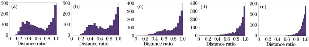
Fig. 2. Histogram of DR in Fig1. (a) 1m2; (b) 1m3; (c) 1m4; (d) 1m5; (e) 1m6

Download full size

Fig. 3. Inliers and outliers in image pairs with zoom^[37]. (a) Image pairs of inliers; (b) distributions of inliers and outliers

Download full size

Fig. 4. Histogram of neighbor inlier distance in Fig. 3. (a) Left image in Fig. 3; (b) right image in Fig. 3

Download full size

Fig. 5. Flow chart of image matching model estimation based on inliers ratio promotion

Download full size

Fig. 6. Identical distribution (ID) and non-identical distribution (NID). (a) ID; (b) NID

Download full size

Fig. 7. Normal distribution of distance between inliers and outliers

Download full size

Fig. 8. Location relationship between undetermined image pairs and inliers

Download full size

Fig. 9. Comparison of time complexity between Ransac and proposed algorithm

Download full size

Fig. 10. Identical distribution matching. (a) Evenly distributed on both images; (b)

Z_{S}

; (c)

Z_{L}

; (d)

Z_{R}

; (e)

Z

Download full size

Fig. 11. Non-identical distribution matching. (a) Left centralization and right dispersion; (b)

Z_{S}

; (c)

Z_{L}

; (d)

Z_{R}

; (e)

Z

Download full size

Fig. 12. Non-identical distributions matching. (a) Left dispersion and right centralization; (b)

Z_{S}

; (c)

Z_{L}

; (d)

Z_{R}

; (e)

Z

Download full size

Fig. 13. Inliers ratio after data filtering

Download full size

Fig. 14. Inliers growth rate

Download full size

Fig. 15. Real images. (a) Wall; (b) Graf1; (c) Graf2; (d) Book; (e) Boat1; (f) Boat2; (g) Valbonne; (h) Bonhall

Download full size

Fig. 16. Change of image pairs’ number

Download full size

Fig. 17. Change of inliers ratio

Download full size

Fig. 18. Comparisons based on homogr data set. (a) Inliers recalls with different distance errors; (b) inliers recalls with different time consumption

Download full size

Fig. 19. Comparisons based on kusvod2 data set. (a) Inliers recalls with different distance errors; (b) inliers recalls with different time comsumption

Download full size

Fig. 20. Inliers recalls of proposed method with different sparsity of matching points. (a) Wall; (b) Graf1; (c) Valbonne

Download full size

Fig. 21. Real images. (a) Booksh; (b) Leafs; (c) Scene0722; (d) Scene0758; (e) Scene0743; (f) Plant; (g) Rotunda; (h) Bread & Toys; (i) Saint Heart

Download full size

Fig. 22. Performance before inliers ratio promotion. (a) Number of pairs of correspondence obtained; (b) ratio of outlier residual; (c) time consumption

Download full size

Fig. 23. Performance after inliers ratio promotion. (a) Number of pairs of correspondence obtained; (b) ratio of outlier residual; (c) time consumption

Download full size

Input： $N$ pairs of correspondences： ${s p_{i}^{L}, s p_{i}^{R}}$ ， $i = 1, 2, \dots, N$

Output： M pairs of correspondences after data filtering： ${s p_{i}^{L}, s p_{i}^{R}}$ ， $i = 1, 2, \dots, M$

Step1： Compute matrix $Z$ according to Eq. （7）， the size of $Z$ is $N \times N$

Step2： Compute the sums of all columns in $Z$ ， and get a data set $K = 255 - \{k_{1}, k_{2}, \dots, k_{N}\}$ ， where $k_{j} = \sum_{i = 1}^{N} z_{i j}$ ， $j = 1, 2, \dots, N$

Step3： Reorder $K$ in ascend， so， a new data set is gotten： $K^{'} = \{k_{1}^{'}, k_{2}^{'}, \dots, k_{N}^{'}\}$ ， in which $k_{j}^{'} \leq k_{j + 1}^{'}$ ， and $j = 1,2, \dots, N$

Step4： Compute the average value of $f$ ： $f = \sum_{j = 1}^{N} k_{j} / N$ ， and then compute $f_{h i g h}$ and $f_{l o w}$ ， where， $f_{l o w} = \sum_{j = 1}^{m^{'}} k_{j}^{'} / m^{'}$ ， $\sum_{j = m^{'} + 1}^{m} k_{j}^{'} / (m - m^{'})$ ， and $m^{'}$ satisfies the expression： $k_{m^{'}}^{'} \leq f \leq k_{m^{'} + 1}^{'}$

Step5： Obtain threshold $T$ ： $T = \{\begin{array}{l} f & i f & f < (f_{l o w} + f_{h i g h}) / 2 \\ (f_{l o w} + f_{h i g h}) / 2 & i f & f \geq (f_{l o w} + f_{h i g h}) / 2 \end{array}$

Step6： Obtain M pairs of correspondences after ${s p_{i}^{L}, s p_{i}^{R}}$ ， where $i$ satisfies the expression： $k_{i}^{'} \geq T$

Table 1. Algorithm of inliers ratio promotion

Input： $N$ pairs of correspondences： $S = \{s p_{i}^{L}, s p_{i}^{R}\}, i = 1, 2, \dots, N$ ； The number of iteration allowed： max itera；termination condition；the initial number of iteration： $i = 1$ ； number of the minimum samples that model can be calculated： $m$ ， 4 （homography）， 7 or 8 （fundamental matrix）

Output： The optimal model or multi models， and its or their inliers

Step1： Obtain the data set $S^{'}$ ， which contains $M$ pairs of correspondences after data filtering as shown in Table 1： $S^{'} = {s p_{i}^{L}, s p_{i}^{R}}$ ， $i = 1, 2, \dots, M$

Step2： $i = i + 1$ ， and sample $m$ pairs of correspondences from $S^{'}$ ， and obtain the current hypothesis $M o_{i}$

Step3： Take $M o_{i}$ to $S$ ， and calculate the number of inliers which are fitted

Step4： Judge whether the hypothesis meets with the termination condition， and whether the current number of iteration meets with max itera， either satisfied， go to Step5， otherwise， return to Step2

Step5： Obtain the optimal model or multi models and its or their inliers

Table 2. Random sample consensus algorithm based on proposed inliers ratio promotion

Input： $N$ pairs of correspondences： $S = \{s p_{i}^{L}, s p_{i}^{R}\}, i = 1, 2, \dots, N$ ； threshold： $T$ ，which is user defined， the type value is 0.01； number of neighbors： $m$ ， which is user defined， and lies in the range from 4 to 6

Output： $S_{i n l i e r s}$

Step1： Obtain the data set $S^{'}$ ， which contains $M$ pairs of correspondences aftering data filtering as shown in Table 1： $S^{'} = {s p_{i}^{L}, s p_{i}^{R}}$ ， $i = 1, 2, \dots, M$ ， and obtain $N - M$ pairs of correspondences which are filtered out： $O = {o_{i}^{L}, o_{i}^{R}}$ ， $i = 1, 2, \dots, N - M$

Step2： Obtain inliers set $S_{i n l i e r s} = {s p_{i}^{L}, s p_{i}^{R}}$ from $S^{'}$ with any graph method， such as NMNET， OANET， PointCN， and SuperGlue， $i = 1, 2, \dots, N_{i n l i e r s}$

Step3： For each pair of correspondence in set $O$ ： ${o_{i}^{L}, o_{i}^{R}}$ ：

1） Obtain the neighbor inliers set that contains $m$ pairs of correspondence with the help of KNN： $p_{1}^{L}, \dots, p_{m}^{L}$ and $p_{1}^{R}, \dots, p_{m}^{R}$ ， and calculate the distance from $O$ to each point of the set： $L_{1}^{L}, \dots, L_{m}^{L}$ and $L_{1}^{R}, \dots, L_{m}^{R}$ ；

2） Normalize the distances by Eq （8）， calculate $d_{e s o}^{L}$ and $d_{e s o}^{R}$ by Eq （9）；

3） Judge whether $d = | d_{e s o}^{L} - d_{e s o}^{R} |$ is not lager than $T$ ， if satisfied， $S_{i n l i e r s} = S_{i n l i e r s} \cup {o^{L}, o^{R}}$ ， and $N_{i n l i e r s} = N_{i n l i e r s} + 1$

End

Table 3. Graph matching algorithm based on proposed inliers ratio promotion

Image	Wall	Graf1	Graf2	Book	Boat1	Boat2	Valbonne	Bonhall
Number of matched pairs	993	2415	2415	1539	3151	3151	1991	1802
Pixel	500×350	800×640	800×640	600×450	850×680	850×680	512×768	490×653
Inliers ratio /%	22.20	15.50	4.10	28.60	30.00	11.30	8.09	19.53

Table 4. Information of image pairs

	OP	PRO	PN	SCR	SC	NAP	MAP	MLE	TDD	OP+	PRO+	PN+	SCR+	SC+	NAP+	MAP+	MLE+	TDD+
Wall	0.43	0.54	0.68	0.78	0.71	0.96	0.91	0.82	0.64	0.22	0.29	0.71	0.54	0.65	0.69	0.62	0.54	0.55
Graf1	1.20	0.66	0.87	1.44	0.94	1.84	1.47	1.66	0.84	0.52	0.43	0.81	0.81	0.84	0.88	0.65	0.80	0.73
Graf2	3.60	0.85	0.57	0.97	0.60	1.49	1.34	1.15	0.79	1.41	0.63	0.72	0.72	0.68	0.76	0.74	0.68	0.72
Book	1.14	0.51	1.01	1.03	1.04	1.68	1.02	1.24	0.58	0.86	0.35	0.55	0.56	0.70	0.74	0.35	0.28	0.50
Boat1	0.74	0.56	1.02	1.83	1.21	2.43	1.87	1.91	0.81	0.71	0.48	0.66	0.92	0.82	0.98	0.61	0.75	0.79
Boat2	3.39	0.23	1.14	1.50	1.34	2.30	1.80	2.10	0.69	0.85	0.25	0.72	0.77	0.81	0.75	0.85	0.74	0.51
Valbonne	2.08	0.54	0.87	1.15	0.50	1.60	1.35	1.30	0.60	1.02	0.32	0.65	0.54	0.49	0.80	0.73	0.64	0.31
Bonhall	3.49	0.41	1.32	1.33	1.05	1.05	1.37	1.04	0.87	1.03	0.77	0.73	0.69	0.74	0.70	0.70	0.70	0.60

Table 5. Comparison of runtime

	OP	PRO	PN	SCR	SC	NAP	MAP	MLE	TDD	OP+	PRO+	PN+	SCR+	SC+	NAP+	MAP+	MLE+	TDD+
Wall	210	190	221	225	223	174	160	150	34	220	229	223	227	225	224	230	233	226
Graf1	365	255	340	330	346	143	147	128	6	370	339	350	341	344	281	340	335	320
Graf2	81	22	51	36	53	20	19	19	6	99	65	79	67	82	51	65	69	36
Book	374	433	433	434	434	368	387	397	179	354	432	433	433	433	428	433	433	433
Boat1	891	958	959	957	958	558	933	937	364	945	958	958	956	958	887	958	957	958
Boat2	296	353	354	353	355	97	64	60	5	343	353	354	353	354	249	347	347	294
Valbonne	132	92	141	112	141	51	51	42	15	145	125	156	127	155	111	127	130	65
Bonhall	300	304	291	317	277	196	233	233	65	336	327	300	321	295	307	327	326	310

Table 6. Comparison of number of obtained inliers

Ruoyan Wei, Junfeng Wang, Xiaoqing Zhu. Inliers Ratio Promotion Algorithm Based on Global Topological Distribution of Image Matching Points[J]. Laser & Optoelectronics Progress, 2022, 59(10): 1010011

Download Citation

Set citation alerts for the article

Tools

Set citation alerts for the article

Save the article for my favorites

Paper Information