The concept of weak measurement [1–4] was introduced by Aharonov, Albert, and Vaidman in 1988. Their theory is based on the von Neumann measurement with a very weak coupling between two quantum systems. Compared to the strong measurement, weak measurement theory is a very important nonperturbative theory of quantum measurements. Over several decades of development, there have been many notable investigations from both fundamental and practical perspectives. On the one hand, weak measurement provides novel insights into a number of fundamental quantum effects, including the role of the uncertainty principle in the Hardy’s paradox [5–7], the double-slit experiment [8,9], the three-box paradox [10], and Leggett-Garg inequalities [11–14]. On the other hand, it is considered to be useful for the signal amplification while decreasing or retaining the technical noise [15,16] in parameter estimations, such as amplification measurements of small transverse [17,18] and longitudinal shifts [19–21], optical nonlinearities [22], and the Poynting vector field [23].

In all these applications, the strange characteristic that the weak value obtained in the weak measurement can even exceed the eigenvalue range of a typical strong or projective measurement and is generally complex (also known as “anomalous weak value”), is usually considered to play a vital role. The standard weak value is defined with post-selection, and the anomalous weak value is usually observed by post-selecting a small subset of data. Therefore, the anomalous weak value is a result of post-selection, which is widely accepted in the community. However there are still great controversies on this point, especially for the validity of weak value technology in quantum metrology [24–26]. With the in-depth research, it is shown that anomalous amplification [27] and unusual smoothed estimation [28] can be realized without the requirement of post-selection of weak measurement techniques in high precise metrology protocols. This result gives us some enlightenments, but it still does not answer the question: can anomalous weak values be attained without post-selection? In fact, it is correct that post-selection is necessary to observe the anomalous weak values in a single weak measurement case. But, it is not the case in general. Recently, a theoretical investigation pointed out that an anomalous weak value can be obtained without post-selection by sequential weak measurements [29,30], which provided a more general insight and was deemed as “yet another surprise” [31].

In this work, we experimentally obtain anomalous weak values in a sequential weak measurement without post-selection, i.e., without discarding any data, in an all-optical system. The photonic polarizations and transverse momenta are chosen to be the system states and pointers, respectively. A sequential weak measurement on the product of two single-qubit observables is realized for arbitrary measurement strength controlled by the phase patterns on a liquid crystal spatial light modulator (SLM). The counter-intuitive average value of joint pointer’s deflection is observed when the measurement strength of the first observable is weak, while the anomalous value disappears when the measurement strength of the first observable increases. Moreover, we further perform a sequential weak measurement on two observables each of which belongs to the components of a two-qubit system and find that an anomalous weak value can never be observed based on commutative sequential weak measurements without post-selection.

The standard form of a weak value is given by which is the mean value of observable A^ when weakly measured between a pre-selected state |ψ⟩ and a post-selected state |f⟩ [1]. As introduced in Refs. [30,32], in particular, a trivial, deterministic measurement of the identity operator I amounts to performing no post-selection. A weak value with no post-selection, can be defined as

Obviously, the weak value with no post-selection is equal to the expectation (average) value of A^. The result of these cases is restricted to lie in [ηmin(A^),ηmax(A^)] (ηmin(max) represents the minimum (maximum) eigenvalue), which means anomalous weak values cannot be observed. It is therefore generally considered that anomalous weak values can only be observed by post-selecting a small subset of data.

However, such an interpretation is invalid for sequential weak measurements [30]. The sequential weak value ⟨(A1A2)ψI⟩W with no post-selection is defined (A^1 and A^2 are independent observables) as follows:

We should note that when A^1 and A^2 are not commute, and for good choices of A1, A2, and |ψ⟩, ⟨(A1A2)ψI⟩W will not be contained within the interval [ηmin(A^1,A^2),ηmax(A^1,A^2)], where ηmin(max)(A^1,A^2)=min(max)k,lηk(A^1)ηl(A^2) (k, l denote the indexes of eigenvalues). Due to the sequential nature of the weak measurements, an anomalous weak value for sequential weak measurements can occur without post-selection.

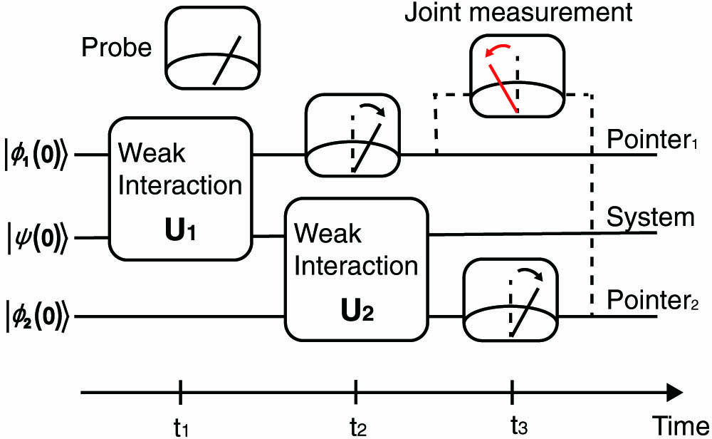
We consider two pointers interacting with a quantum system one after another as illustrated in Fig. 1. Suppose a qubit system initially prepared in the general state |ψ⟩, while two-pointer states are prepared in |ϕ1⟩ and |ϕ2⟩, respectively. The evolution operator between the system and pointer is denoted as U^i=exp(iγiA^i⊗F^i), where i∈{1,2} denotes the ith weak measurement, γi is the interaction coupling, and F^i is an operator of the pointer. The result of the sequential weak measurements can be linked to the anomalous weak value without post-selection ⟨(A1A2)ψI⟩W.

Specifically, let us consider a qubit system initially prepared in the state |ψ⟩=|0⟩, assuming A^i to be the projection observable on the system with A^i=|ai⟩⟨ai|, where |ai⟩=12|0⟩−(−1)i32|1⟩, and to each measurement is associated a momentum operator F^i=p^i of the pointers. Considering a Gaussian pointer [33] with transverse wavefunction ϕi=exp(−x2/σi2) (σi is a constant), the joint pointer average position is given by [30] where x^i represents the ith position operator. Here we define the inferred values of M=⟨x^1⊗x^2⟩/γ1γ2. Since each output pointer observable has an average shift in the range of [0,1], the average values are naturally expected within the range [0,1]. However, when the first measurement is sufficiently weak, γ1→0, ⟨x^1⊗x^2⟩≈−18γ1γ2 lied out of the interval, which shows the average product of the pointer displacements is proportionally linked to the anomalous weak value, where M→Re[⟨(A1A2)ψI⟩W]=−18. Interestingly, in the real weak limit, as γ1→0, then ⟨x^1⊗x^2⟩→0 also, unless γ2 is increased to compensate it. In contrast, when the first measurement is strong (γ1→∞), ⟨x^1⊗x^2⟩≈116γ1γ2 is consistent with the product of the two observables’ expectation values, where M→⟨ψ|A1|ψ⟩|⟨a1|a2⟩|2=116.

We experimentally demonstrate sequential weak measurements [34] by using the SLM, in which a phase φ (φ=αr→mod2π, α∈N) that changes linearly along the r→ direction is implemented to the input photons. The evolution can be described as where p^r→=−i∂∂r→ (setting ℏ=1) represents the momentum operator, |H⟩ represents the horizontal polarization of the photon, and γexp=kα(k∈R) represents the coupling strength which can be conveniently tuned by changing the blazing density of the hologram on the SLM (see Appendices A and B for more details). We set γ1=γ2=γexp in the experiment.

In the experiment, the photon’s polarizations and transverse field momenta (p^x→,p^y→) are chosen to be the system A^i and pointers F^i, respectively. The experimental setup is illustrated in Fig. 2(a). Single photons (SPs) from an intrinsic defect in a GaN crystal are filtered by a single mode fiber [35] (see Appendices A and B for more details). The zero-delay time of the second-order correlation function g2(0) is measured to be 0.262 and fitted to be 0.025, which clearly demonstrates the single photon property.

A half-wave plate (HWP1) with the optical axis set to be 30° is used to prepare the polarization state of the photon to be |a1⟩=12|H⟩+32|V⟩, where |V⟩ represents the vertical polarization. Then the photons are focused on the right screen of SLM for the first weak coupling by a convex lens with a focal length of 150 mm. The hologram loaded on the right area of SLM is a vertical blazed grating, and satisfies φright(x,y)=αx→mod2π(α∈N). In the experiment, γexp=0.0237α (see Appendices A and B for details). This progress can be defined as U^1=exp(iγexpA^1⊗p^x→).

Similarly, through a lens with a focal length of 75 mm, photons are re-focused on the left screen of SLM for the second weak coupling, and the evolution becomes U^2=exp(iγexpA^2⊗p^y→). The left hologram is a horizontal grating, which satisfies φleft(x,y)=αy→mod2π. Another HWP2 with the optical axis set to be −30° is placed before the screen to rotate |H⟩(|V⟩) to the state of |a2⟩=12|H⟩−32|V⟩(|a2⊥⟩=32|H⟩−12|V⟩). The third Fourier lens is used to translate the photons back to the coordinate space, which are directly detected by an intensified charge coupled device (ICCD) without post-selection of polarizations.

Figure 2(b) shows several spatial distributions of the photons with different coupling strengths. The scale of images is 1024×1024 and the pixel length is 13.5 μm. The coupling strength γexp varies from 0 to 0.37 mm. When γexp is less than 0.1 mm, the coupling strength is so small that the transverse coordinate deflection is much less than the Rayleigh distance. With the increase of coupling strength, the deflections of the transverse coordinates are clearly observed, including downward deflection ϕ(x+γexp,y), rightward deflection ϕ(x,y+γexp) and down-rightward deflection ϕ(x+γexp,y+γexp) after sequential weak measurements U^1 and U^2, respectively. The insets in Fig. 2(b) show the theoretical output patterns, of which the similarity is quantitatively determined by the correlation value (Corr) [36] compared with the experimental images. The Corr is larger than 0.96 when γexp>0.2366; the errors are mainly due to the aberrations in optical systems and the inaccuracy of wave plate rotation.

To quantitatively describe the anomalous weak values, we define the transverse coordinate pointer’s position ⟨K^⟩ as the mean of the transverse field coordinate as follows: where K^∈{x^,y^,x^⊗y^}. ϕ′(x,y) is the final photonic transverse wave function and x^⊗y^ represents the joint pointer position operator [37]. The result of the sequential measurement is proportional to the product of the pointer positions.

Figure 3 shows the deflection of the pointer as a function of the coupling strength. The coupling strength γexp varies from 0 to 0.711 mm. The pointer positions of horizontal and vertical transverse coordinates (⟨x^⟩ and ⟨y^⟩) are shown in Fig. 3(a) with the brown and blue dots representing the experimental results and the brown and blue lines representing the corresponding theoretical predictions, respectively. No matter what the coupling strength is, we can find that ⟨x^⟩ and ⟨y^⟩ is larger than 0. The joint pointer positions ⟨x^⊗y^⟩ are shown in Fig. 3(b). The green dots represent the experimental results with the green line representing the corresponding theoretical prediction. Anomalous phenomenon ⟨x^⊗y^⟩<0 can be observed when the coupling strength γexp is less than 0.331 mm, which is shown as the red dots. When γexp=0.189mm, the reversed deflection of the joint pointer reaches the maximum. The values are smaller than prediction, which may be due to the slight tilt of the ICCD camera and the optical aberrations. The error bars represent the corresponding standard deviation [Δ(⟨x^⊗y^⟩)]. Figure 3(c) shows the inferred values of M=⟨x^⊗y^⟩/γexp2. When γexp→0, M equals the real part of the weak value Re[⟨(A1A2)ψI⟩W]=−18. However, the experimental errors Δ(⟨x^⊗y^⟩)/γexp2 also get amplified with γexp→0, which makes the inferred weak values get unreliable. In spite of this, when 0.13mm<γexp<0.3mm, M still approximates to the anomalous weak value −18, and the experimental tendency here is consistent with the theoretical prediction.

Moreover, as a comparison, considering the situation of a sequential weak measurement of two observables, which are measured on each of two qubits respectively, there is no such anomalous deflection at all. Supposing a sequential measurement of the commuting observables A^1⊗I and I⊗A^2 is performed on the bipartite system, the average weak value is equal to the expectation value of A^1⊗A^2 in the absence of any post-selection, with ⟨(A^1⊗A^2)ψI⟩W=⟨ψ|A^1⊗A^2|ψ⟩, which can never exceed the range of eigenvalues of the observable.

We experimentally investigate the case of weak measurement on two individual photons, which corresponds to the sequential weak measurement on different parts of a bipartite system. We first apply the U^1 to a photon and obtain the deflection of the pointer’s positions in the x direction (⟨x^⟩). We then implement the U^2 to the other photon and obtain the deflection of the pointer’s positions in the y direction (⟨y^⟩). The experimental results of ⟨x^⟩ (brown dots) and ⟨y^⟩ (blue dots) with the corresponding theoretical predictions represented as brown and blue lines, respectively, are shown in Fig. 4(a). The experimental results of the joint pointer deflection ⟨x^⊗y^⟩ (green dots) and the corresponding theoretical prediction (green line) are shown in Fig. 4(b), in which the values of ⟨x^⊗y^⟩ are all larger than zero. Error bars represent the corresponding standard deviations. All position deflections are larger than zero and satisfy ⟨x^⟩=⟨y^⟩=⟨x^⊗y^⟩. There is not any anomalous phenomenon for sequential weak measurement with any coupling strength for two qubit systems, since the two observables are commutative in the sequential case.

We have experimentally carried out a sequential measurement of two observables in a single-qubit system and a two-qubit system for arbitrary measurement strength with the SLM. The anomalous weak values are obtained without post-selection, in which the paradox of average pointer deflection is successfully observed in a single-qubit system. Such an anomalous phenomenon disappears when the measurement strength of the first observable becomes strong. On the other hand, when a sequential weak measurement is commutative, the anomalous weak value can never be observed without post-selection.

The experimental method of sequential weak measurement is implemented by taking the photon polarizations and transverse field momenta as the system and pointers, respectively. Compared with other methods [38,39], the advantage of this approach is that the coupling strength can be conveniently adjusted, so one can obtain weak values at different coupling strengths.

The tendencies of experimental data coincide with the theoretical predictions. Since the region to detect deflections of photon distributions associated with the anomalous weak value is less than 10−3mm2, the output results are easily disturbed. Moreover, the error of weak values will be rapidly increased as the coupling strength decreases. This effect can be mitigated by increasing γ2. This would give an idea of the tradeoff between the fact that, theoretically, one obtains a more anomalous weak value the further one goes to the weak regime, and the fact that the observable effect also becomes smaller in the weak limitation.

By controlling their measurement strengths from weak to strong, different results of a sequential measurement of two observables in weak and strong limits have been clearly shown. The anomalous weak values emerge in the sequential weak measurements. Recently, weak values and sequential weak measurements have played crucial roles in understanding fundamental problems such as the information paradox in black holes [40–43], time [44], and geometric phase [45]. The sequential measurement technology demonstrated in this work may be useful for exploring a series of fundamental physical concepts.

Acknowledgment. This work was partially carried out at the USTC Center for Micro and Nanoscale Research and Fabrication.