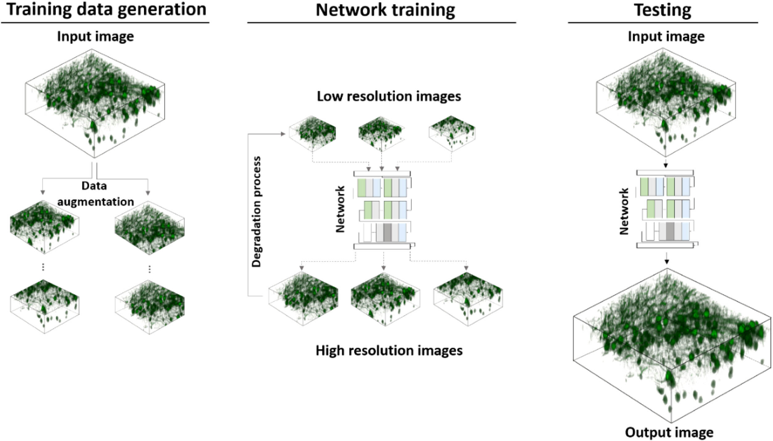
Fig. 1. Overview of proposed framework. The input image is first cropped and augmented into patches. The downsampled version of the patches is then used as the input for training, where the original patches serve as the target output. At the test phase, the input image is fed to the trained network to produce high-resolution output.

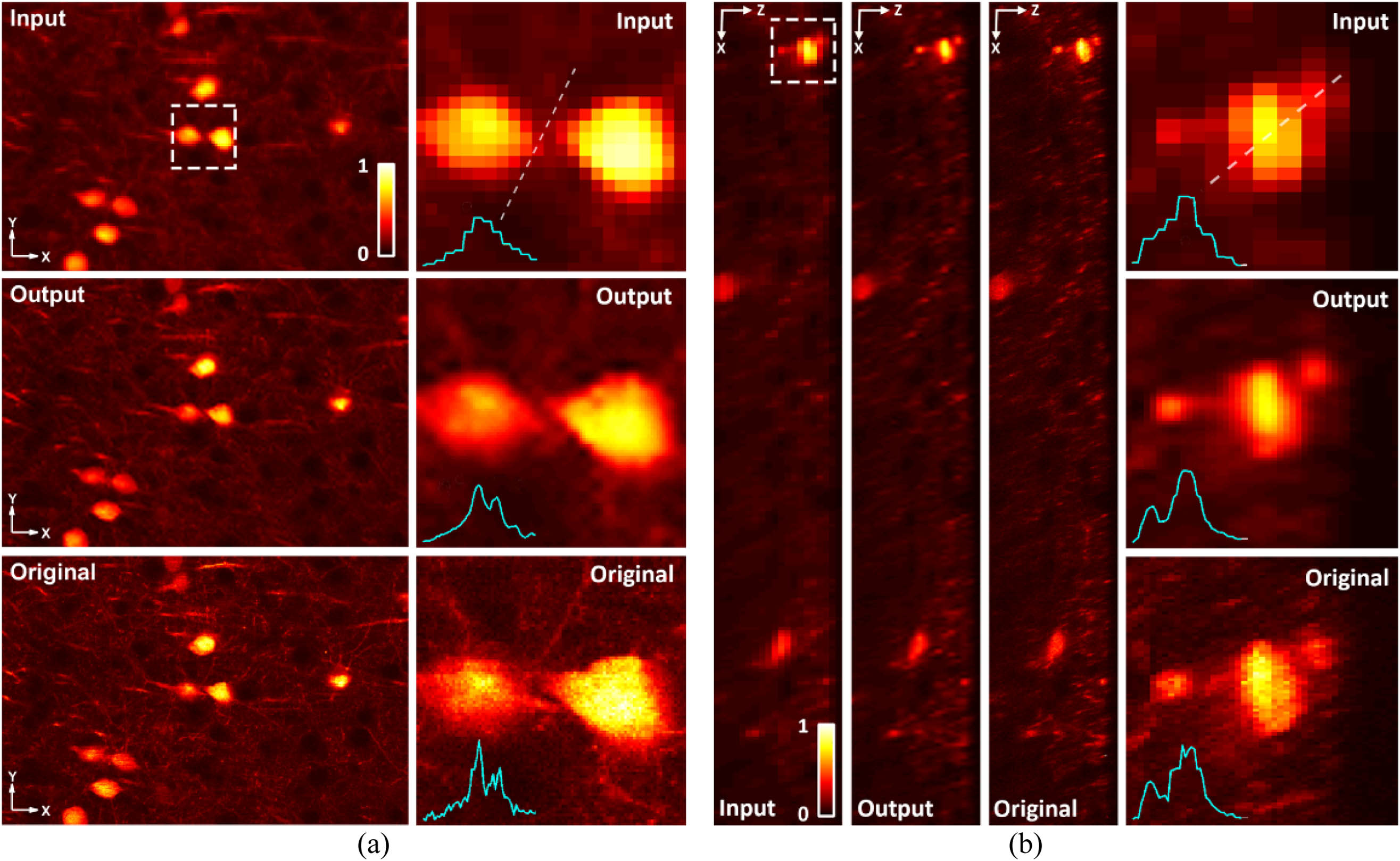
Fig. 2. Zoomed-in images of neurons and their line profiles across the white dashed line. (a) Lateral images. (b) Axial images.

Fig. 3. Evaluation of four super-resolution models. Lateral and axial images of low-resolution input, original reference, and network outputs of neuron cells. Our proposed model shows low error. (a) Representative lateral images inferred from low-resolution input. The absolute error images with respect to the original are shown below. (b) Representative axial images inferred from low-resolution input.

Fig. 4. PSNR and SSIM evaluation between the four models.

Fig. 5. Large image inference using a high-resolution input. High-resolution image (1024×1024  px) can still benefit from the network (details shown on the right-hand side of the inset). The downsampled low-resolution version of the same input with its network enhanced image is shown on the left-hand side of the inset for comparison.

Fig. 6. Volumetric image inference using a high-resolution input. Top left: input lateral slice; top right: corresponding output slice; bottom left: input axial slice; bottom right: corresponding output slice.

Fig. 7. Large image inference of Self-Vision (image brightness adjusted for visualization). Despite being trained on a small FOV (indicated by yellow border), Self-Vision can infer the entire FOV for the system, saving both training and acquisition time.

Fig. 8. Network performance improves as the training FOV increases. At the top left corner, the boxes with small, medium, and large sizes indicate different input training volumes (not drawn to scale). The plot at the top right shows that network performance improves as the voxel number increases. The bottom images [(c)–(j) lateral, (k)–(p) axial] illustrate the change of the output when the training FOV increases from a small volume to a large volume.

Fig. 9. Architecture of Self-Vision. Some grouped convolution layers were omitted in the figure for simplicity.

Table 1. Summary of Parameters Related to Network Training for Performance Comparison