Self-supervised deep-learning two-photon microscopy

Yuezhi He; Jing Yao; Lina Liu; Yufeng Gao; Jia Yu; Shiwei Ye; Hui Li; Wei Zheng

doi:10.1364/PRJ.469231

Abstract

Artificial neural networks have shown great proficiency in transforming low-resolution microscopic images into high-resolution images. However, training data remains a challenge, as large-scale open-source databases of microscopic images are rare, particularly 3D data. Moreover, the long training times and the need for expensive computational resources have become a burden to the research community. We introduced a deep-learning-based self-supervised volumetric imaging approach, which we termed “Self-Vision.” The self-supervised approach requires no training data, apart from the input image itself. The lightweight network takes just minutes to train and has demonstrated resolution-enhancing power on par with or better than that of a number of recent microscopy-based models. Moreover, the high throughput power of the network enables large image inference with less postprocessing, facilitating a large field-of-view (

2.45 mm \times 2.45 mm

) using a home-built two-photon microscopy system. Self-Vision can recover images from fourfold undersampled inputs in the lateral and axial dimensions, dramatically reducing the acquisition time. Self-Vision facilitates the use of a deep neural network for 3D microscopy imaging, easing the demanding process of image acquisition and network training for current resolution-enhancing networks.

1. INTRODUCTION

Two-photon excitation fluorescence microscopy (TPM) [1] is a powerful tool for 3D imaging of cellular and subcellular structures and functions deep in turbid tissues. Owing to its nonlinear excitation properties, TPM provides compelling performance of near-diffraction-limited spatial resolution in deep and scattered samples. However, conventional TPM captures volumetric images by serially scanning the focal point in a 3D space [2], which requires compromises among the imaging resolution, speed, and area [3]. A higher-resolution image requires a higher number of sequentially acquired pixels to ensure proper sampling, thus increasing the imaging time. Considerable effort has been devoted to speeding up the acquisition efficiency of imaging systems, such as multifocal scanning [4], temporal focusing [5], and multiplane imaging [6]. However, these methods modify the light path and require sophisticated hardware design. Developing a new method to effectively enhance undersampled point-scanning TPM images is of great practical interest for biological studies.

Deep learning [7], a method based on artificial neural networks (ANNs), has drawn wide-spread attention among the microscopy research community and has been used for segmentation and recognition in microscopy image analysis. In recent years, various new applications have emerged, including modality transformation [8], image denoising at a low photon budget [9], reducing light exposure for TPM [10], accelerating single-molecule localization [11], speeding up multicolor spectroscopic single-molecule localization microscopy [12], 3D virtual refocusing [13], and instantaneous fluorescence lifetime calculation [14,15]. Among numerous others [16 –19], super-resolution imaging via a deep neural network [20], which transforms spatially undersampled images into super-sampled ones, is one of the hottest topics. It tackles this problem by training the network to learn the mapping between low-resolution images and their high-resolution counterparts [21]. When low-resolution images are presented, the network is expected to output or infer a high-resolution image with high fidelity. Using deep-learning-based image-enhancing techniques, high-resolution images can now be recovered from low-resolution images with reduced scan times and no hardware modifications.

The majority of deep neural networks used in microscopic imaging rely on training with hundreds of thousands of high-quality images [3,8,20,22]. For the image-resolution-enhancement task, high-resolution images are paired with corresponding low-resolution images for supervised network training. However, large-scale 3D online microscopic image databases are limited. Moreover, training with data generated from different systems may cause performance changes owing to data drift. Consequently, most research is based on self-collected image pairs. Low-resolution images can be acquired experimentally, followed by careful image registration [20], or by simply applying a degradation model to digitally downsample high-resolution images [3,23,24]. The long acquisition process inevitably incurs high costs. Recent research has shown the estimated cost of acquiring 240 h of high-resolution electron microscopic imaging data to be over $8000 [24]. The cost doubles if low-resolution images are measured experimentally. Acquiring 3D data worsens the situation, as the sample preparation is different, and imaging time significantly increases, not to mention the potential risks of photobleaching. In addition to the cost of data acquisition, the computational cost is non-negligible. The large neural networks routinely used in current deep learning microscopy not only require a large volume of data to fit but also require high-performance computing resources, such as high-end graphical processing units (GPUs) or cloud-based computing platforms, to train, which is an additional burden for many optical and biomedical laboratories.

Sign up for Photonics Research TOC. Get the latest issue of Photonics Research delivered right to you！Sign up now

In this study, we developed a lightweight model to enhance the resolution of 3D microscopic images. The model requires zero training data apart from the input volumetric image itself; therefore, it is fully self-supervised [25 –27], i.e., Self-Vision. We demonstrated that Self-Vision could recover images, while the input was fourfold undersampled in both the lateral and axial dimensions, which in theory results in an over 60-fold ( $4 \times 4 \times 4$ ) reduction in the actual acquisition time, although there is some degradation of image quality. We also compared Self-Vision with multiple recent networks specifically developed for enhancing microscopic images and found that our proposed framework achieved fewer errors and greater structural similarity using only the input image for training. Furthermore, we applied the framework to a home-built large field-of-view (FOV) imaging system. Using only a small portion of the image cropped from the entire FOV for training, the network reconstructed a high-resolution image with more than a significant reduction in the volumetric acquisition time.

2. RESULTS

A. Concept of Self-Supervised Resolution-Enhanced Volumetric Image

Figure 1 shows the concept of Self-Vision-based resolution-enhancement for volumetric images. The image pairs for training are generated by first cropping small patches from the input image (training data generation in Fig. 1) and then downsampling the patches along with their augmentations to synthesize low-resolution inputs (network training in Fig. 1). After the training stage, the input image is sent to the network for a high-resolution output. To avoid confusion with super-resolution techniques using optical methods, we use the term “resolution-enhancing” instead for deep-learning-based methods throughout the work. Some combinations (e.g., super-resolution network/model) are kept, which are consistent with the common expressions in the literature.

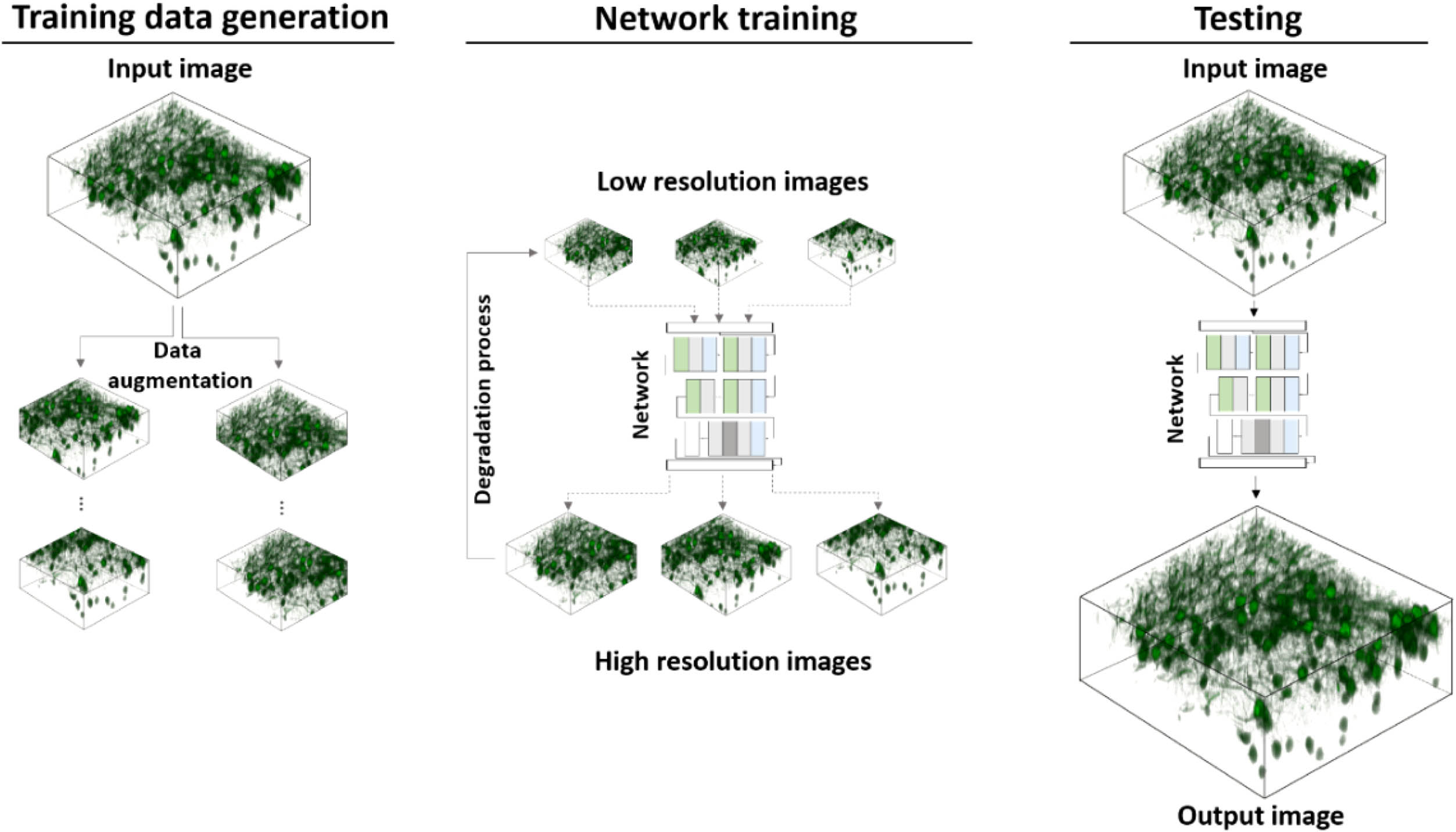
Overview of proposed framework. The input image is first cropped and augmented into patches. The downsampled version of the patches is then used as the input for training, where the original patches serve as the target output. At the test phase, the input image is fed to the trained network to produce high-resolution output.

Figure 1.Overview of proposed framework. The input image is first cropped and augmented into patches. The downsampled version of the patches is then used as the input for training, where the original patches serve as the target output. At the test phase, the input image is fed to the trained network to produce high-resolution output.

In the context of volumetric image enhancement, the patches can be extracted from a single input image scale of the order of $N^{3}$ , serving as the data source for the self-supervised learning process (Fig. 1, left). This data-saving training strategy does not rely on a massive training data set, i.e., it removes the burden of collecting a large-scale training set, as both the number and size of training data are reduced. Once the model is trained, it can be deployed for inference purposes (see Supplementary Fig. S1 in Ref. [28]) for a comparison between the two data-training strategies. Meanwhile, the lightweight, minimalistic model allows a large input image, thereby favoring images captured using a large FOV system and alleviating the stitching process in postprocessing. Finally, network training can be completed within minutes, thus considerably reducing the total cost.

B. Self-Vision Improves Resolution of Undersampled Volumetric Images

Using a microscope, the process of sampling a volumetric image, $V_{Original} (x, y, z)$ , can be formulated using the classical image degradation model: $V_{L.R.} = (V_{Original} * PSF) ↓_{n},$ (1)where $V_{L.R.}$ represents the acquired low-resolution image, PSF is the system point spread function, and $↓_{n}$ is the downsampling factor, which is usually determined by an image-capturing device, such as a charge-coupled device (CCD) camera or photomultiplier tube.

Our goal was to train a neural network, $F$ , to transform the input $V_{L.R.}$ to its high-resolution, de-pixelated version, $V_{H.R.} = F (V_{L.R.})$ such that $V_{H.R.}$ was as close as possible to the ground-truth $V_{Original}$ .

To demonstrate the efficacy of our Self-Vision network, we first used simulated beads (see Supplementary Fig. S2 in Ref. [28] and Methods) with anisotropic profiles. The reference image, $V_{Original}$ , was artificially generated, and the input, $V_{L.R.}$ , was obtained via downsampling. Using the proposed framework, both the lateral and axial profiles of the output agreed with the reference image (see Supplementary Figs. S2 and S3 in Ref. [28]). These results demonstrated that Self-Vision recovered the bead profile when the input was fourfold undersampled in the lateral and axial dimensions, indicative of a reduction in the actual acquisition time.

We then verified whether Self-Vision could improve the resolution of undersampled volumetric images acquired from real biological samples and infer details that were undistinguishable in the degraded inputs using a commercially available microscope (Nikon A1R-MP). The networks were trained and tested using 3D images of green fluorescent protein (GFP) labelled Thy-1 brain slices from mice (see Section 4). The brain slices were placed on glass slides for two-photon microscopy using a $25 \times$ , 1.1 NA water immersion objective (N25X-APO-MP, Nikon). The excitation wavelength was set to 920 nm, and the neurons could be clearly visualized. To test the network performance, a high-resolution reference image was captured from a $520 μm \times 520 μm \times 152 μm$ ( $X \times Y \times Z$ ) volume with a lateral spacing of 0.51 μm and an axial spacing of 1 μm. This resulted in an output image size of $1024 \times 1024 \times 152$ voxels.

Figure 2 shows Self-Vision TPM imaging of neurons from the mouse brain tissue. The neuron bodies from the test specimens are magnified and shown, along with the intensity profiles drawn from a line across the image (marked by a white dash). In the lateral and axial dimensions, the network outputs have a similar profile to the original image (the contrast between the cells and the background also being enhanced). For example, the troughs between the two peaks, i.e., the blue line profile plots in Fig. 2, which show little contrast on the input profile, become distinguishable in the output profile. An unexpected feature of the network is that the output images appear less noisy than the original images, as the spatially undersampled inputs filter out any high-frequency noise (caused by system instability or background noise) and content present in the original images.

Figure 2.Zoomed-in images of neurons and their line profiles across the white dashed line. (a) Lateral images. (b) Axial images.

C. Comparison with Representative Deep-Learning-Based Super-Resolution Models

We chose three representative deep-learning-based super-resolution models with different designs for microscopic images for comparison (see Methods section Supplementary Note 2 in [28] for data preparation and network training), including a recent attention-based network (DFCAN) [29], which uses Fourier domain information and outperforms a number of classical super-resolution networks; a network designed for point-scanning microscopy (PSSR) [24], which trains on computationally degraded low-resolution images; further, it should be noted that our framework shares the same method of generating undersampled images; and a super-resolution model with a dual-stage processing architecture (DSP-Net) [23], which also supports 3D input like our method. These models require much more data than our network for training (see Supplementary Fig. S1 in [28], data-hungry training). Consequently, in addition to the test images, four extra regions of similar volume (size) were collected from the specimen using the same device to train the three representative models used for microscopic image resolution enhancement. The low-resolution input for training could be either experimentally acquired from the same regions or synthetically generated by downsampling. Experimentally, we found that it was difficult to register low-resolution–high-resolution image pairs at subpixel-level precision, which is generally required for super-resolution image training. In addition, sample instability and laser power fluctuations complicate postprocessing. Consequently, low-resolution images were synthetically generated by downsampling the reference images. In total, over 500 additional high-resolution images were acquired to train the models for comparison (see Section 4). By contrast, our framework used no additional training data, the only input being the volume to be inferred. Even so, our model exhibited excellent performance. Practically, our framework has a great advantage in that there is no need to image hundreds of high-quality images for training data, as the low-resolution input image can be directly fed to the network to obtain a high-resolution output. It should be noted that training with a larger data set may improve the performance of other networks, but this just proves that our training strategy is effective, especially when the sample is rare or the training data are limited.

Figure 3(a) shows the low-resolution input, network outputs, and original high-resolution reference from a lateral slice of the test sample. It should be noted that DFCAN and PSSR are 2D super-resolution networks; therefore, the volumetric images were fed to the network slice by slice. Our framework and DSP-Net support 3D images. The input slice shown in Fig. 3(a) is $256 \times 256$ pixels, and the edges of the neuron cells appear rough and blocky. All inferred images show improved smoothness across the entire image. To visualize the difference between the inferred images and the original image, absolute error maps ( $| Output - Original |$ ) are shown beneath the model outputs. It is clear that our network outputs the smallest error, the cell body of the neurones being inferred well. A close inspection of our error map reveals that many errors originate from filament-like fine details in the axon or background. It is difficult to recover such details because the input is highly undersampled ( $4 \times$ in all dimensions).

Figure 3.Evaluation of four super-resolution models. Lateral and axial images of low-resolution input, original reference, and network outputs of neuron cells. Our proposed model shows low error. (a) Representative lateral images inferred from low-resolution input. The absolute error images with respect to the original are shown below. (b) Representative axial images inferred from low-resolution input.

Figure 3(b) shows the inferred results from the axial slice of the test sample. Because both our network and DSP-Net allow volumetric inputs and utilize 3D information, the axial output error is much smaller than that of the 2D networks DFCAN and PSSR. Another error source of a 2D network is the improper normalization of deeper slices. As a deeper slice receives fewer photons, the image brightness tends to decrease. Inferring the output in a slice-by-slice manner using a 2D network can overamplify the overall brightness in the deeper layers and cause noticeable errors. Consequently, we statistically measured the performance of the networks using the peak signal-to-noise ratio (PSNR) and structural similarity (SSIM). The box plots shown in Fig. 4 were calculated using 32 sets of samples. Our network outperforms the others in both metrics, thereby confirming the effectiveness of the proposed framework.

Figure 4.PSNR and SSIM evaluation between the four models.

D. Large-Image Inferencing Using Self-Vision

Having seen the potential of using a self-supervised Self-Vision network to enhance spatially undersampled images (see Fig. 2), we next exploited an important feature of our lightweight framework, i.e., inferring large input images.

In many well-known super-resolution models for microscopic images, a common problem is that the input image size is limited; for example, for a typical input size $(256 \times 256 px$ ) with $4 \times$ resolution-enhancement, the output size is limited to $1024 \times 1024 px$ because large neural networks consume a substantial amount of GPU memory. This limitation complicates postprocessing and compromises the quality of the output image, as large images must be cropped into smaller patches for inference, which can cause boundary artefacts.

Benefitting from the lightweight design, our framework supports $4 \times$ resolution-enhancement using a 2D input size of $1024 \times 1024 px$ (output size of $4096 \times 4096 px$ ) and a 3D input size of $256 \times 256 \times 21 px$ (output size of $1024 \times 1024 \times 84 px$ , see Supplementary Fig. S4 in Ref. [28]) with a single-pass inference, surpassing both the 2D and 3D models previously compared. We first demonstrated the application of large-image inference to enhance high-resolution images using Self-Vision. Figure 5 shows a high-resolution image ( $1024 \times 1024 px$ ); the inset shows two sets of network-enhanced results obtained using our network.

Figure 5.Large image inference using a high-resolution input. High-resolution image ( $1024 \times 1024 px$ ) can still benefit from the network (details shown on the right-hand side of the inset). The downsampled low-resolution version of the same input with its network enhanced image is shown on the left-hand side of the inset for comparison.

On the left-hand side of the inset image, a low-resolution image generated from downsampling is enhanced. This is a typical application of most deep-learning-based networks (see Visualization 1). However, most published models fail to enhance high-resolution images that contain many pixels owing to the aforementioned size constraint. On the right-hand side of the Fig. 5 inset, we show an enlarged region of a high-resolution image ( $1024 \times 1024 px$ ) and its network-enhanced result. The output can be inferred in a single forward pass without stitching (see Visualization 2).

Figure 6 shows the results from a volumetric input ( $256 \times 256 \times 38 px$ ). An interesting feature of the network is its nonlinearity, the different cells having different output intensities. This is because the 3D network considers neighboring axial slices, and the output intensity changes accordingly, depending on the adjacent axial slices (see Visualization 3 and Visualization 4).

Figure 6.Volumetric image inference using a high-resolution input. Top left: input lateral slice; top right: corresponding output slice; bottom left: input axial slice; bottom right: corresponding output slice.

E. Large Field-of-View TPM Imaging Based on Self-Vision

To demonstrate how Self-Vision enhances undersampled images (which we believe is the most useful case of the network), we developed a home-built large-FOV system (see Section 4 for the system configuration). Generally, a large-FOV system suffers from a slow imaging process. This can be detrimental to the sample because of phototoxicity or photobleaching. Moreover, slow acquisition decreases the temporal resolution, making transient phenomena difficult to observe. Consequently, we applied our framework to images acquired using a large-FOV system. The image size was $1024 \times 1024 px$ with a lateral step size of $Δ x$ or $Δ y = 2.4 μm$ , corresponding to a volume of $2.45 mm \times 2.45 mm$ . Point scanning of such a volume at the Nyquist rate would require a long imaging period. Therefore, the step size was intentionally set to be larger than the Nyquist criteria, so that the imaging time could be reduced, and we could verify whether the image resolution could be improved by Self-Vision at a sub-Nyquist sampling rate.

Figure 7 shows the power of Self-Vision in large-image inference. Using only a small training FOV (bounded by the yellow border in Fig. 7), the network can infer the full FOV (bounded by the blue border in Fig. 7) in a single forward pass. No cropping of the input or stitching of the outputs is required; thus, data processing for images captured from a large-FOV system can be greatly simplified.

Figure 7.Large image inference of Self-Vision (image brightness adjusted for visualization). Despite being trained on a small FOV (indicated by yellow border), Self-Vision can infer the entire FOV for the system, saving both training and acquisition time.

3. DISCUSSION

Despite the tremendous success of the deep-learning-based method used in the microscope imaging community, the high cost of computational resources and the demand for large-scale training data remain practical challenges. Our deep learning-based approach improves the resolution of spatially undersampled microscopic images with zero training data (apart from the input image itself), which can be useful in a data-limited scenario, such as investigating pathological sections from rare diseases. In such cases, gathering hundreds of training data points from similar specimens is a luxury that medical practitioners cannot afford. By exploiting the internal information present in a single low-resolution image, we can achieve performance on par with that of multiple state-of-the-art models trained using hundreds of additional paired data. Another advantage of the Self-Vision framework is that it facilitates large-FOV imaging. Despite being trained with only a small portion of the image from the entire view, Self-Vision can infer a high-resolution image for the entire FOV. This can substantially reduce the acquisition time for large-FOV systems, as high-resolution images that would otherwise require a long time to sample can be inferred from a spatially undersampled version. Moreover, the lightweight model allows large images to be inferred with less image cropping/stitching, easing the processing of high-dimensional images.

Nevertheless, it is important to keep in mind that deep-learning-based super-resolution is naturally ill-posed. Consequently, the output represents only a statistical estimation of the training data. In practice, the following points must be considered. First, hallucinations or artefacts become overwhelming when the upsampling factor goes beyond $4 \times$ , as when the input image is contaminated by system noise, the network may amplify the noise as well. Meanwhile, small details, such as dendrites as thin as 1–2 px on the high-resolution image, are bound to be lost when downsampled. In this case, it can be impossible to recover these features faithfully. In addition, the self-supervised training scheme may result in performance changes when the test sample originates from a different domain. For better performance, training a new network is recommended if there is a significant shift in the input data type. With our small-sized model, we believe that transferring the trained model to new sample types can be easily realised.

It is worth noting that the size of the input image can affect the network performance because the only source of training data is the input image itself. For instance, if the input image is too small, even with data augmentation, the patches generated may still be limited, and the model is likely to be overfitted. However, if the input image is too large, our small-sized model may struggle to further improve the input, owing to the limited model parameters. To determine the appropriate input size, we trained the model using images of different input sizes and examined its performance. Seven volumes of different voxel numbers were cropped from the center of the test image [Fig. 8(a)].

Figure 8.Network performance improves as the training FOV increases. At the top left corner, the boxes with small, medium, and large sizes indicate different input training volumes (not drawn to scale). The plot at the top right shows that network performance improves as the voxel number increases. The bottom images [(c)–(j) lateral, (k)–(p) axial] illustrate the change of the output when the training FOV increases from a small volume to a large volume.

The smallest input was $64 \times 64 \times 8 px$ , and the largest input size was $256 \times 256 \times 38 px$ (see Section 4 for details). Compared with images inferred from a small training FOV [Figs. 8(e) and 8(f)], the outputs from a large training FOV [Figs. 8(g) and 8(h)] show lower background noise. Statistical analysis of the SSIM and PSNR (see Supplementary Note 3 in Ref. [28]) shown in Fig. 8(b) reveals that, when the input voxel number is greater than $1 \times 10^{5}$ , the performance of the proposed model starts to level off. This size corresponds to an input image size of $100 \times 100 \times 10 px$ , which can easily be satisfied for ordinary 3D imaging. Generally, the number of training patches extracted from a volumetric sample is proportional to the cube of its input dimensions. By contrast, for the 2D samples, the cubic relationship reduces to a quadratic relationship. Consequently, a model with more parameters would favor the volumetric input size because more patches could be extracted for training.

Future work should focus on the following aspects. Our current design improves spatial resolution; however, the time dimension remains unexplored. The proposed framework could increase the frame rate of sparsely sampled 3D video data by adding additional dimensions to the network. Another effort could be to integrate a sophisticated downsampling method into the data augmentation process. As only the naïve downsampling method is used to synthesize low-resolution images, the system noise and point spread function are ignored. Adding an accurate estimation of these factors to the downsampling process could further improve the network performance. Moreover, designing a network that could be trained without a modern GPU would be of great practical interest because the majority of microscopes are not equipped with high computing power.

Taken together, the lightweight design, data-saving training strategy, and high-throughput capability of the Self-Vision framework represent an important step for computational super-resolution imaging. Our ability to bridge the gap between neural network training and microscopic image acquisition is key to democratizing deep-learning-based super-resolution imaging. We expect the framework to continue to develop, not only in the modalities used in this work but also in various imaging modalities for different tasks, as the barriers to applying deep learning in microscopy are continually lowered.

4. METHODS

A. Simulation of Bead Images

All the reference bead images were generated using MATLAB. First, a 3D matrix of size $512 \times 512 \times 60$ filled with zeroes was defined. To generate beads in the matrix, 500 random points in the matrix were set to one. This step simulated the point sources in space. A 3D anisotropic point spread function was then created via the built-in function “fspecial3.” The TYPE, HSIZE, and SIGMA arguments were set to “Gaussian,” [19 19 19], and [2 2 4], respectively. Finally, the 3D matrix was convolved with the point spread function using the “convn” function to create original images. The low-resolution input images for network training were generated using the Python built-in function “rescale” from the skimage package, with SCALE set to 0.25 and the other parameters kept to their default values. The function works by first convolving the input image with a 3D Gaussian filter to avoid aliasing and then downsampling the convolved image. The process corresponds to the acquisition of a low-resolution image using a microscope, which downsampled the original images four times in all dimensions, resulting in images of size $128 \times 128 \times 15.$ A line across the center of the bead was extracted to calculate its full width at half maximum (FWHM). MATLAB’s “fit” function with FITTYPE “gauss1” was then used to fit the line profile. The FWHM was calculated to be $2.355 \times σ$ , where the $σ$ represents the standard deviation of the fitted line.

B. Mouse Brain Slices Preparation

A six-week-old mouse (The Jackson Laboratory, stock number 007788) labelled with the Thy1-GFP-M transgene, which is intensely expressed in mossy fibers in the cerebellum, was first anaesthetized by intraperitoneal injection with a mixture of 2% $α$ -chloralose and 10% urethane (8 mL/kg). Before fixation, the mouse was perfused transcranially using phosphate-buffered saline (PBS) and 4% (w/v) paraformaldehyde (PFA). The mouse was then sacrificed, its brain being carefully excised from its skull for overnight fixation with 4% PFA. Finally, 2 mm thick slices were obtained from the brain using a custom-made sectioning mold. The CX3-GFP labelled mouse brain slices used in the large-image inference experiments were prepared in the same manner. The sectioned samples were then placed on a glass slide and covered with a coverslip for microscopic imaging.

C. Microscope Setup and Imaging Parameters

Two microscopes were used for the imaging experiments. One was a commercially available two-photon microscope (Nikon A1R), and the other was a home-built large FOV two-photon microscope. The light source of the system in the Nikon A1R is a Ti:sapphire laser (MaiTai eHP DeepSee, Spectra Physics), which can generate an excitation wavelength of 920 nm for two-photon imaging. The laser power was set to 2.8 with a gain of 110. A $25 \times$ , 1.1 NA water-immersion objective (N25X-APO-MP, Nikon) was chosen to acquire the volumetric imaging data. The original image size used for the model comparison shown in Fig. 7 is $1024 \times 1024 \times 152$ , corresponding to a volume of $520 μm \times 520 μm \times 152 μm$ , as the voxel size was set to $0.51 μm \times 0.51 μm \times 1 μm$ . To generate low-resolution images, the original images were first convolved using the system point spread function (PSF), which could be calculated from the numerical aperture (NA) of the objective and the excitation wavelength, and then digitally downsampled. A faster implementation uses the “cubic” resize function. Both implementations produced similar results in the experimental settings.

To acquire additional training data for the other networks, four extra volumes of similar sizes were imaged. The lateral image size was still $1024 \times 1024$ , the axial size varying between 152 and 162, depending on the sample thickness. Some slices near the top or bottom imaging volume were discarded because no useful signal could be acquired at those positions. This resulted in 543 slices of 2D images used to train the comparison networks (see Supplementary Note 2 in Ref. [28]). Note that one of the comparison networks, i.e., DSP-Net, supports 3D resolution enhancement; therefore, volumetric data from the same data source were used for training. The acquisition time for a single volume was approximately 20 min.

For the home-built large-FOV two-photon microscopy, the detailed implementation of the large-FOV TPM used can be found in Ref. [30]. In short, we applied an adaptive-optics method to extend the FOV, resulting in an increased FOV diameter of 3.46 mm using a commercial objective with a nominal FOV diameter of 1.8 mm.

D. Self-Supervised Volumetric Image Super-Resolution Network

The design of our Self-Vision network follows two principles. First, the network needs to be trained using only a single volumetric input instance. Second, the model supports large-image inference. To fulfil these requirements, a small neural network was devised. Figure 9 shows the network architecture of the proposed design. The network is composed of four modules, i.e., extraction, shrinking, grouped convolution, and expansion. It begins with feature extraction for the input with 3D convolution using a filter size of 5 and a parametric rectified linear unit (PReLU) activation layer. Formally, PReLU can be expressed as follows: $PReLU (y_{i}) = y_{i}, if y_{i} \geq 0,$ (2) $PReLU (y_{i}) = a_{i} \leq y_{i}, if y_{i} < 0,$ (3)where $y_{i}$ is the layer output and $a_{i}$ is a learnable parameter.

Figure 9.Architecture of Self-Vision. Some grouped convolution layers were omitted in the figure for simplicity.

The output of the extraction module can be expressed as follows: $y_{expansion} = PReLU [Conv 3 d_{1, 16, 5} (x)],$ (4)where $x$ represents the input image, and $Conv 3 d_{1, 16, 5}$ is the 3D convolution kernel with an input channel of 1, an output channel of 16, and a size of $5 \times 5 \times 5$ .

Consequently, the shrinking module reduces the number of filters from 16 to 6 using filters of size 3. The output of the shrinking module can be expressed as follows: $y_{shrinking} = PReLU [Conv 3 d_{16, 6, 3} (y_{expansion})] .$ (5)

Subsequently, multiple layers of grouped convolution, followed by PReLU activation, can be used to further extract high-level features. This can be expressed as follows: $y_{grouped convolution} = Conv 3 d_{6, 6, 3, 2}^{(4)} (y_{shrinking}),$ (6)where $Conv 3 d_{6, 6, 3, 2}^{(4)}$ represents four layers of 3D convolution operations, with each layer using six input channels, six output channels, a kernel size of 3, and grouped by two.

The expansion module then upsamples the output from the previous layer to the desired resolution. In this step, subpixel convolution is used as the upsampling operation in conjunction with 3D convolution to create a high-resolution image. Finally, multiple images are fused using backprojection techniques to create a monochromatic network output. Consequently, the output of the neural network can be expressed as follows: $y_{output} = Conv 3 d_{16, 1, 5} {UP [Conv 3 d_{6, 16, 3} (y_{grouped convolution})]},$ (7)where UP is the subpixel convolution layer responsible for upsampling.

Several designs are critical for the network to work well, and the shrinking and grouped convolution modules substantially reduce the total number of network parameters, making single-input data training feasible. The super-resolution network employs a post-super-resolution upsampling framework, where the computation-intensive feature extraction process takes place in the low-dimensional space, greatly lowering the space and computational complexity. The subpixel convolution used for upsampling and the backprojection technique further reduces the output error.

Learning the end-to-end mapping network, $F$ , for super-resolution requires estimation of the network parameters, $θ$ . This is done by optimizing the loss function (also known as the objective function) between the inferred outputs, $F (x, θ)$ , and the target images, $Y$ . The mean squared error (MSE) can be used as the loss function, as it measures the pixel-wise difference between the network output and the target. The MSE can be expressed as follows: $MSE (θ) = \frac{1}{n} \sum_{i = 1}^{n} {[F (x, θ) - Y]}^{2},$ (8)where $Y$ is the target volumetric output, $F (x, θ)$ represents the network predictions, and $n$ is the number of training samples. The network parameters can be optimized using the standard gradient descent with backpropagation. Although only the MSE is formally optimized, alternative evaluation metrics, such as SSIM and PSNR, can be simultaneously improved through training.

E. Self-Vision Implementation

The network was written in Python using the PyTorch software (the source code is publicly available at https://github.com/frankheyz/s-vision). The three networks were also trained for comparison using their open-source code, which can be found in the references. Table 1 summarizes the key parameters related to network training. All networks were trained on a PC of the following specifications: Intel Xeon E5-2678 W CPU, 256 GB RAM, and a single NVIDIA TITAN X GPU. Our network used a minimum amount of training data (see Supplementary Note 1 in Ref. [28] for data augmentation and training) and achieved excellent quantitative performance. The training time of a single volumetric input was just 6 min, which is substantially shorter than that of the other methods. 2D and 3D images could be inferred by our network, demonstrating a clear advantage over 2D super-resolution networks. Moreover, the 3D inference speed was fast because the small-sized network could infer large input images quickly with fewer stitches.Table 1.

Summary of Parameters Related to Network Training for Performance Comparison

Methods	Modality	Training Image Size	Training Data Size	Training Time	2D Inference $(1024 \times 1024)$	3D Inference $(1024 \times 1024 \times 152)$
DFCAN	Nikon A1R-MP	$1024 \times 1024 \times 152 \times 4$	0.6 GB	2.5 h	0.2 s	N/A
PSSR				1.2 h	0.6 s	N/A
DSP-Net				11.2 h	N/A	120 s
Ours		$256 \times 256 \times 38$	N/A	6 min	0.5 s	62 s

Acknowledgment

Acknowledgment. We thank Dr. H. Zhang, Dr. S. Wang, and Dr. S. He for assistance and discussion with algorithm development and evaluation.

References

[1] W. Denk, J. H. Strickler, W. W. Webb. Two-photon laser scanning fluorescence microscopy. Science, 248, 73-76(1990).

[2] J. Wu, N. Ji, K. K. Tsia. Speed scaling in multiphoton fluorescence microscopy. Nat. Photonics, 15, 800-812(2021).

[3] M. Weigert, U. Schmidt, T. Boothe, A. Müller, A. Dibrov, A. Jain, B. Wilhelm, D. Schmidt, C. Broaddus, S. Culley, M. Rocha-Martins, F. Segovia-Miranda, C. Norden, R. Henriques, M. Zerial, M. Solimena, J. Rink, P. Tomancak, L. Royer, F. Jug, E. W. Myers. Content-aware image restoration: pushing the limits of fluorescence microscopy. Nat. Methods, 15, 1090-1097(2018).

[4] T. Zhang, O. Hernandez, R. Chrapkiewicz, A. Shai, M. J. Wagner, Y. Zhang, C. H. Wu, J. Z. Li, M. Inoue, Y. Gong, B. Ahanonu, H. Zeng, H. Bito, M. J. Schnitzer. Kilohertz two-photon brain imaging in awake mice. Nat. Methods, 16, 1119-1122(2019).

[5] E. Papagiakoumou, E. Ronzitti, V. Emiliani. Scanless two-photon excitation with temporal focusing. Nat. Methods, 17, 571-581(2020).

[6] D. R. Beaulieu, I. G. Davison, K. Kılıç, T. G. Bifano, J. Mertz. Simultaneous multiplane imaging with reverberation two-photon microscopy. Nat. Methods, 17, 283-286(2020).

[7] Y. Lecun, Y. Bengio, G. Hinton. Deep learning. Nature, 521, 436-444(2015).

[8] H. Wang, Y. Rivenson, Y. Jin, Z. Wei, R. Gao, H. Günaydın, L. A. Bentolila, C. Kural, A. Ozcan. Deep learning enables cross-modality super-resolution in fluorescence microscopy. Nat. Methods, 16, 103-110(2019).

[9] J. Chen, H. Sasaki, H. Lai, Y. Su, J. Liu, Y. Wu, A. Zhovmer, C. A. Combs, I. Rey-Suarez, H. Y. Chang, C. C. Huang, X. Li, M. Guo, S. Nizambad, A. Upadhyaya, S. J. J. Lee, L. A. G. Lucas, H. Shroff. Three-dimensional residual channel attention networks denoise and sharpen fluorescence microscopy image volumes. Nat. Methods, 18, 678-687(2021).

[10] S. McAleer, A. Fast, Y. Xue, M. J. Seiler, W. C. Tang, M. Balu, P. Baldi, A. W. Browne. Deep learning-assisted multiphoton microscopy to reduce light exposure and expedite imaging in tissues with high and low light sensitivity. Transl. Vis. Sci. Technol., 10, 30(2021).

[11] W. Ouyang, A. Aristov, M. Lelek, X. Hao, C. Zimmer. Deep learning massively accelerates super-resolution localization microscopy. Nat. Biotechnol., 36, 460-468(2018).

[12] S. Kumar Gaire, Y. Zhang, H. Li, R. Yu, H. F. Zhang, L. Ying. Accelerating multicolor spectroscopic single-molecule localization microscopy using deep learning. Biomed. Opt. Express, 11, 2705-2721(2020).

[13] Y. Wu, Y. Rivenson, H. Wang, Y. Luo, E. Ben-David, L. A. Bentolila, C. Pritz, A. Ozcan. Three-dimensional virtual refocusing of fluorescence microscopy images using deep learning. Nat. Methods, 16, 1323-1331(2019).

[14] J. T. Smith, R. Yao, N. Sinsuebphon, A. Rudkouskaya, N. Un, J. Mazurkiewicz, M. Barroso, P. Yan, X. Intes. Fast fit-free analysis of fluorescence lifetime imaging via deep learning. Proc. Natl. Acad. Sci. USA, 116, 24019-24030(2019).

[15] R. Yao, M. Ochoa, P. Yan, X. Intes. Net-FLICS: fast quantitative wide-field fluorescence lifetime imaging with compressed sensing: a deep learning approach. Light Sci. Appl., 8, 26(2019).

[16] Y. Rivenson, H. Wang, Z. Wei, K. de Haan, Y. Zhang, Y. Wu, H. Günaydın, J. E. Zuckerman, T. Chong, A. E. Sisk, L. M. Westbrook, W. D. Wallace, A. Ozcan. Virtual histological staining of unlabelled tissue-autofluorescence images via deep learning. Nat. Biomed. Eng., 3, 466-477(2019).

[17] X. Li, G. Zhang, H. Qiao, F. Bao, Y. Deng, J. Wu, Y. He, J. Yun, X. Lin, H. Xie, H. Wang, Q. Dai. Unsupervised content-preserving transformation for optical microscopy. Light Sci. Appl., 10, 44(2021).

[18] L. Huang, H. Chen, Y. Luo, Y. Rivenson, A. Ozcan. Recurrent neural network-based volumetric fluorescence microscopy. Light Sci. Appl., 10, 62(2021).

[19] L. Jin, Y. Tang, Y. Wu, J. B. Coole, M. T. Tan, X. Zhao, H. Badaoui, J. T. Robinson, M. D. Williams, A. M. Gillenwater, R. R. Richards-Kortum, A. Veeraraghavan. Deep learning extended depth-of-field microscope for fast and slide-free histology. Proc. Natl. Acad. Sci. USA, 117, 33051-33060(2020).

[20] Y. Rivenson, Z. Göröcs, H. Günaydin, Y. Zhang, H. Wang, A. Ozcan. Deep learning microscopy. Optica, 4, 1437-1443(2017).

[21] C. Dong, C. C. Loy, X. Tang. Accelerating the super-resolution convolutional neural network. European Conference on Computer Vision, 391-407(2016).

[22] L. Jin, B. Liu, F. Zhao, S. Hahn, B. Dong, R. Song, T. C. Elston, Y. Xu, K. M. Hahn. Deep learning enables structured illumination microscopy with low light levels and enhanced speed. Nat. Commun., 11, 1934(2020).

[23] H. Zhang, Y. Zhao, C. Fang, G. Li, M. Zhang, Y.-H. Zhang, P. Fei. Exceeding the limits of 3D fluorescence microscopy using a dual-stage-processing network. Optica, 7, 1627-1640(2020).

[24] L. Fang, F. Monroe, S. W. Novak, L. Kirk, C. R. Schiavon, S. B. Yu, T. Zhang, M. Wu, K. Kastner, A. A. Latif, Z. Lin, A. Shaw, Y. Kubota, J. Mendenhall, Z. Zhang, G. Pekkurnaz, K. Harris, J. Howard, U. Manor. Deep learning-based point-scanning super-resolution imaging. Nat. Methods, 18, 406-416(2021).

[25] M. Zontak, M. Irani. Internal statistics of a single natural image. Proceedings of the IEEE Computer Society Conference on Computer Vision and Pattern Recognition, 977-984(2011).

[26] A. Shocher, N. Cohen, M. Irani. Zero-shot super-resolution using deep internal learning. Proceedings of the IEEE Computer Society Conference on Computer Vision and Pattern Recognition, 3118-3126(2018).

[27] X. Li, G. Zhang, J. Wu, Y. Zhang, Z. Zhao, X. Lin, H. Qiao, H. Xie, H. Wang, L. Fang, Q. Dai. Reinforcing neuron extraction and spike inference in calcium imaging using deep self-supervised denoising. Nat. Methods, 18, 1395-1400(2021).

[28] Y. He, J. Yao, L. Liu, Y. Gao, J. Yu, S. Ye, H. Li, W. Zheng. Self-supervised deep-learning two-photon microscopy: supplemental document.

[29] C. Qiao, D. Li, Y. Guo, C. Liu, T. Jiang, Q. Dai, D. Li. Evaluation and development of deep neural networks for image super-resolution in optical microscopy. Nat. Methods, 18, 194-202(2021).

[30] J. Yao, Y. Gao, Y. Yin, P. Lai, S. Ye, W. Zheng. Exploiting the potential of commercial objectives to extend the field of view of two-photon microscopy by adaptive optics. Opt. Lett., 47, 989-992(2022).